Overland Flow
Overland flow simulates the movement of ponded surface water across the topography. It can be used for calculating flow on a flood plain or runoff to streams.
You can run the Overland flow module separately, or you can combine it with any of the other modules. However, overland flow is required when you are using a river model in MIKE SHE, as the overland flow module provides lateral runoff to the rivers.
The Simplified Overland Flow Routing method can be used for regional applications when detailed flow is not required. This method assumes that ponded water in the upland areas of a subcatchment flows into the flood plain areas of the subcatchment, which in turn discharges uniformly into the stream network located in the subcatchment.
The Finite Difference Method uses the diffusive wave approximation and should be used when you are interested in calculating local overland flow and runoff. There are two solution methods available.
The choice of method is a tradeoff between accuracy and solution time. The SOR solver is generally faster because it can run with larger time steps. The Explicit method is generally more accurate than the SOR method but is often constrained to smaller time steps. The time step constraint prevents flow from crossing a cell in a single time step. The time step constraint is determined by the cell with the highest velocity and applied to the entire model in the current time step.
The Explicit method is generally used when the river is allowed to spill from the river onto the flood plain. Alternatively, you can use Flood codes to inundated flood plain areas based on the water level in the river.
The Multi-grid overland flow option allows you to take advantage of detailed DEM information if it is available. The multi-grid method, sub-divides the overland flow cell into an even number of sub-cells. The gradients between the cells and the flow area between cells water surface elevation in the cell is then calculated based on the volume of water and the detailed topography information.
In MIKE SHE, the calculation of 2D overland flow can become a very time-consuming part of the simulation. So, you need to be very careful when setting up your model to minimize the calculation of overland flow between cells when it is unnecessary.
Detailed information on Overland Flow, the coupling between MIKE 1D and MIKE SHE and the overbank spilling options, and ways to optimize the calculation of overland flow can be found in the chapters:
Manning’s M
The Manning M is equivalent to the Stickler roughness coefficient, the use of which is described in Overland Flow - Technical Reference.
The Manning M is the inverse of the more conventional Manning’s n. The value of n is typically in the range of 0.01 (smooth channels) to 0.10 (thickly vegetated channels). This corresponds to values of M between 100 and 10, respectively. Generally, lower values of Manning’s M are used for overland flow compared to channel flow.
If you don’t want to simulate overland flow in an area, a Manning’s M of 0 will disable overland flow. However, this will also prevent overland flow from entering into the cell.
Detention Storage
Detention Storage is used to limit the amount of water that can flow over the ground surface. The depth of ponded water must exceed the detention storage before water will flow as sheet flow to the adjacent cell. For example, if the detention storage is set equal to 2mm, then the depth of water on the surface must exceed 2mm before it will be able to flow as overland flow. This is equivalent to the trapping of surface water in small ponds or depressions within a grid cell.
If you have static ponded water in an area and you do not want to calculate overland flow between adjacent cells (can be slow), then you can set the detention storage to a value greater than the depth of ponding.
Water trapped in detention storage continues to be available for infiltration to the unsaturated zone and to evapotranspiration.
Initial and Boundary Conditions
In most cases it is best to start your simulation with a dry surface and let the depressions fill up during a run in period. However, if you have significant wetlands or lakes this may not be feasible. However, be aware that stagnant ponded water in wetlands may be a significant source of numerical instabilities or long run times.
The outer boundary condition for overland flow is a specified head, based on the initial water depth in the outer cells of the model domain. Normally, the initial depth of water in a model is zero. During the simulation, the water depth on the boundary can increase and the flow will discharge across the boundary. However, if a non-zero value is used on the boundary, then water will flow into the model as long as the internal water level is lower than the boundary water depth. The boundary will act as an infinite source of water.
If you need to specify time varying overland flow boundary conditions, you can use the Extra Parameter option Time-varying Overland Flow Boundary Conditions.
Separated flow areas
The Separated Flow Areas are typically used to prevent overland flow from flowing between cells that are separated by topographic features, such as dikes, which cannot be resolved within the grid cell.
If you define the separated flow areas along the intersection of the inner and outer boundary areas, MIKE SHE will keep all overland flow inside of the model, making the boundary a no-flow boundary for overland flow.
1. Overland Drainage and Paving
Overland drainage (OL Drainage) is a special boundary condition in MIKE SHE used to define natural and artificial drainage systems that cannot be captured by the River Network. This is an effective means to specify urban drainage networks and large-scale upland drainage areas.
OL Drainage is taken from rainfall and ponded water on the cell. Water that is removed is routed to local surface water bodies, local topographic depressions, or out of the model. The amount of drainage is calculated based on the depth of ponding, rainfall and the drain level using a linear reservoir formulation.
When water is removed from a drain, it is immediately moved to the OL Drain Storage. In other words, the drain module assumes that the time step is longer than the time required for the drainage water to move to the storage. From the OL Drain Storage, the water is released to the recipient at a rate based on the discharge time constant.
Each cell requires a drain level, inflow time constant (which is the same as a leakage factor, optional), and an outflow time constant. Both drain levels and time constants can be spatially distributed. The default drainage level is the topography. A typical time constant may be between 0.01 and 0.00001 1/s.
Drainage reference system
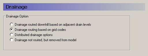
MIKE SHE requires a reference system for linking the drainage to a recipient node or cell. There are four different options for setting up the drainage source-recipient reference system.
Drain Levels
The drainage recipient is calculated based on the drain levels in all the down gradient cells. That is, the location of the recipient cell is calculated as if the drain water was flowing downhill (based on the drain levels). This is the most common method of specifying drainage routing and the default setting.
Drain Codes
The drainage recipient is specified by the user based on a distribution map of integer code values.
Distributed option
With this option there are several different drainage possibilities, including a combination of Codes and Levels. The Distributed option can also be used to define a specific river H-point or sewer manhole as a recipient.
Removed
The fourth option is simply a head dependent boundary that removes the drainage water from the model.
2. Multi-cell overland flow
The main idea behind the 2D, multi-cell solver is to make the choice of calculation grid independent of the topographical data resolution. The approach uses two grids:
- One describing the rectangular calculation grid, and
- The other representing the fine bathymetry.
The standard methods used for 2D grid-based solvers do not make a distinction between the two. Thus, only one grid is applied, and this is typically chosen based on a manageable calculation grid. The available topography is interpolated to the calculation grid, which typically does not do justice to the resolution of the available data. The 2D multi-grid solver in MIKE SHE can, in effect, use the two grids more or less independently.
In the Multi-cell overland flow method, high resolution topography data is used to modify the flow area used in the St Venant equation and the courant criteria. The method utilizes two grids - a fine-scale topography grid and a coarser scale overland flow calculation grid. However, both grids are calculated from the same reference data - that is the detailed topography digital elevation model.
In the Multi-cell method, the principle assumption is that the volume of water in the fine grid and the coarse grid is the same. Thus, given a volume of water, a depth and flooded area can be calculated for both the fine grid and the coarse grid.
In the case of detention storage, the volume of detention storage is calculated based on the user specified depth and OL cell area.
During the simulation, the cross-sectional area available for flow between the grid cells is an average of the available flow area in each direction across the cell. This adjusted cross-sectional area is factored into the diffusive wave approximation used in the 2D OL solver. For numerical details see Multi-cell Overland Flow Method in the Reference manual.
The multi-grid overland flow solver is typically used where an accurate bathymetric description is more important than the detailed flow patterns. This is typically the case for most inland flood studies. In other words, the distribution
of flooding and the area of flooding in an area is more important than the rate and direction of ingress.
The multi-grid option is described in more detail in the chapter Multi-cell Overland Flow.
3. Overland Flow Performance
Calculation of overland flow can be a significant source of numerical instabilities in MIKE SHE. Depending on the model setup, the overland flow time step can become very short, making the simulation time very long.
The chapter Surface Water in MIKE SHE contains many more details on simulating overland flow and the coupling to MIKE 1D. In particular the section Overland Flow Performance contains detailed information on improving the performance of the overland flow in your model.
4. MIKE+ 2D Overland
MIKE SHE provides a useful means to simulate 2D flooding on a flood plain that includes the influence of infiltration and evapotranspiration. However, the detailed simulation of surface water flow paths and velocities on a flood plain can be very difficult. If you need to simulate more complex flood plain flow, for example the impact of flood plain structures and embankments, you may need to use the 2D Overland module in MIKE+ instead of MIKE SHE.
The MIKE+ 2D Overland module enables coupling of the 2D MIKE 21FM surface water model for detailed, accurate flow on the flood plain with MIKE 1D for channel flow. MIKE+ allows you to define flood plain structures such as embankments and culverts that can have very significant impacts on flow velocity and direction. The MIKE 21FM engine can also more accurately simulate flood wave propagation on a surface simply because of the higher order numerical method used.