Getting Started

Introduction

In the hydrological cycle, water evaporates from the oceans, lakes, and rivers, from the soil and is transpired by plants. This water vapour is transported in the atmosphere and falls back to the earth as rain and snow. It infiltrates to the groundwater and discharges to streams and rivers as base flow. It also runs off directly to streams and rivers that flow back to the ocean. The hydrologic cycle is a closed loop and our interventions do not remove water; rather they affect the movement and transfer of water within the hydrologic cycle.

MIKE SHE is an advanced, flexible framework for hydrologic modelling. It includes a full suite of pre- and post-processing tools, plus a flexible mix of advanced and simple solution techniques for each of the hydrologic processes. MIKE SHE covers the major processes in the hydrologic cycle and includes process models for evapotranspiration, overland flow, unsaturated flow, groundwater flow, and channel flow and their interactions. Each of these processes can be represented at different levels of spatial distribution and complexity, according to the goals of the modelling study, the availability of field data, and the modeller’s choices. The MIKE SHE user interface allows the user to intuitively build the model description based on the user's conceptual model of the watershed. The model data is specified in a variety of formats independent of the model domain and grid, including native GIS formats. At run time, the spatial data is mapped onto the numerical grid, which makes it easy to change the spatial discretisation.

MIKE SHE uses MIKE+ Rivers to simulate channel flow. MIKE+ includes comprehensive facilities for modelling complex channel networks, lakes and reservoirs, and river structures, such as gates, sluices, and weirs. In many highly managed river systems, accurate representation of the river structures and their operation rules is essential. In a similar manner, MIKE SHE is also linked to the MIKE+ Collection Systems (formerly known as MOUSE) sewer model, which can be used to simulate the interaction between urban storm water and sanitary sewer net-works and groundwater. MIKE SHE is applicable at spatial scales ranging from a single soil profile, for evaluating crop water requirements, to large regions including several river catchments, such as the 80,000 km2 Senegal Basin. MIKE SHE has proven valuable in hundreds of research and consultancy projects covering a wide range of climatological and hydrological regimes.

The need for fully integrated surface and groundwater models, like MIKE SHE, has been highlighted by several independent studies. These studies show that few codes exist that have been designed and developed to fully integrate surface water and groundwater. Further, few of these have been applied outside of the academic community.

MIKE SHE has been used in a broad range of applications. It is being used operationally in many countries around the world by organisations ranging from universities and research centres to consulting engineers companies. MIKE SHE has been used for the analysis, planning and management of a wide range of water resources and environmental and ecological problems related to surface water and groundwater, such as:

• River basin management and planning
• Water supply design, management and optimisation
• Irrigation and drainage
• Soil and water management
• Surface water impact from groundwater withdrawal
• Conjunctive use of groundwater and surface water
• Wetland management and restoration
• Ecological evaluations
• Groundwater management
• Environmental impact assessments
• Aquifer vulnerability mapping
• Contamination from waste disposal
• Surface water and groundwater quality remediation
• Floodplain studies
• Impact of land use and climate change

Impact of agriculture (irrigation, drainage, nutrients and pesticides, etc.)

The MIKE SHE user interface

MIKE SHE’s user interface can be characterised by the need to

• Develop a GUI that promotes a logical and intuitive workflow, which is why it includes
• A dynamic navigation tree that depends on simple and logical choices
• A conceptual model approach that is translated at run-time into the mathematical model
• Object oriented “thinking” (geo-objects with attached properties)
• Full, context-sensitive, on-line help

Customised input/output units to support local needs

• Strengthen the calibration and result analysis processes, which is why it includes
• Default HTML outputs (calibration hydrographs, goodness of fit, water balances, etc.)
• User-defined HTML outputs
• A Result Viewer that integrates 1D, 2D and 3D data for viewing and animation

Water balance, auto-calibration and parameter estimation tools.

• Develop a flexible, unstructured GUI suitable for different modelling approaches, which is why it includes
• Flexible data format (gridded data, .shp files, etc.) that is easy to update for new data formats
• Flexible time series module for manipulating time-varying data

Flexible engine structure that can be easily updated with new numerical engines

The result is a GUI that is flexible enough for the most complex applications imaginable, yet remains easy-to-use for simple applications.

In addition to the MIKE ZERO Project Explorer, the MIKE SHE document consists of 4 parts:

• Along the top - the Tool bar and drop-down Menus
• On the left - the dynamic Data tree and tab control
• In the middle - the context sensitive Dialog area
• On the right - the Project Explorer

Along the bottom - the Validation area and Mouse-over data area

Tool bar - contains icon short cuts for many MIKE SHE operations that can be accessed via the Menus. The Tool bar changes depending on the tools that are currently in use.

Data tree - displays the data items required to run the model as it is currently defined. If you add or subtract hydrologic processes or change numeric engines, the make-up of the data tree will change.

Dialog area - is different for each item in the data tree.

Validation area - displays information on missing data or invalid data items. Any items displayed here are hot linked to the Dialog in which the error has occurred.

Mouse-over area - displays dynamic coordinate and value information related to the mouse position in the map area of any of the spatial Dialogs.

Project Explorer - displays the list of files that are in the current project. This is only active if the model is opened and edited via a Project File. Otherwise the section is blank.

Setting up a MIKE SHE Flow Model

The purpose of this exercise is to set up an integrated MIKE SHE model using predefined inputs. Through the exercise, basic MIKE SHE operations are practised and you will become familiar with various model tools for result processing.

The exercise is divided into two parts.

This section covers the following topics:

• Creating a model
• Setting up the model domain and grid
• Adding the topography
• Specifying climate and land use
• Setting up the various modules: overland, unsaturated and saturated flow; and
• Controlling the outputs.

The second part, Section 4, covers

• Running the model, and
• Using some of the post-processing tools to evaluate the results

The models in these exercises are based on the Karup River catchment in western Denmark.

Create a new MIKE SHE setup

In the following steps you will be creating and building a new MIKE SHE model of the catchment based largely on pre-existing data files.

Ensure that you have installed the Example files in the previous Getting Started exercise

Create a new MIKE SHE document

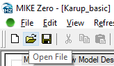
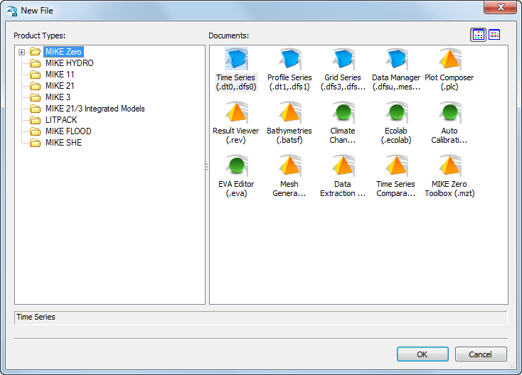
All of the MIKE Powered by DHI documents can be created from the File\New\File... menu in the top pull-down menu or by clicking on the New File icon, , in the toolbar.

When the New File Dialog appears,

• select MIKE SHE in the bottom of the list on the left hand side,
• select Flow Model (.she) on the right hand side,
• click OK.

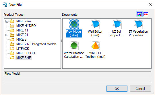
The default MIKE SHE Setup Dialog will now appear.

The .SHE file contains all the user-specified information required to run MIKE SHE. However, the file does not contain the actual time series and grid data. MIKE SHE only stores the path names to the other data files for time-series data and grid data. This greatly improves the flexibility of the user interface for keeping your model up-to-date with new data and for running calibration and prediction scenarios

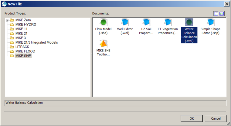
You can use the same New document dialog to select any of the listed file types on the right hand side, or even navigate to one of the other items on the left hand side. For example, you may need to create a water balance (.wbl) file during calibration, or a new dfs0 time series file, which you will find under the MIKE Zero list.

Save the document file

The document file that you just created – in this case the .she document – is unnamed until you save it.

To save the file:

• Use the File\Save menu item, or the Save icon
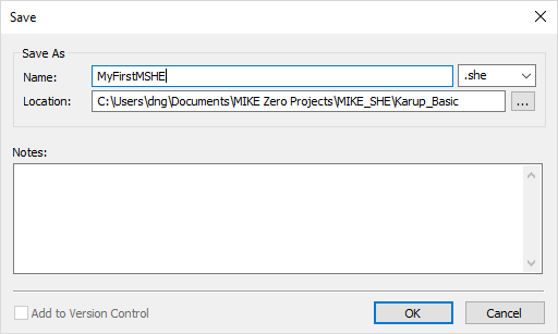
• In the Save Dialog type in a file name (e.g. Karup_Basic1 or MyFirstMSHE – the .she extension will be added automatically)

Click OK

Set up the map overlays

In many projects, the first thing you may want to do is to define the maps and overlays that you are going to use in your project.

MIKE SHE allows you to add graphical overlays using bitmaps, tiffs, ArcView .shp files, etc. These overlays will appear on all maps shown in the graphical view in the user interface.

Set the display area

The basic display area of the model map view is defined in the top item of the data tree Dialog under Display:

Use your mouse pointer to select Display

The Display item is located at the top of the data tree to make it easy to add and edit your background maps. In the Display item, you can add any number of images to your model setup, in a variety of formats. The images are carried over to the various editors, so you can keep a consistent display between the set up editor and, for example, the Grid Editor and the Results Viewer.

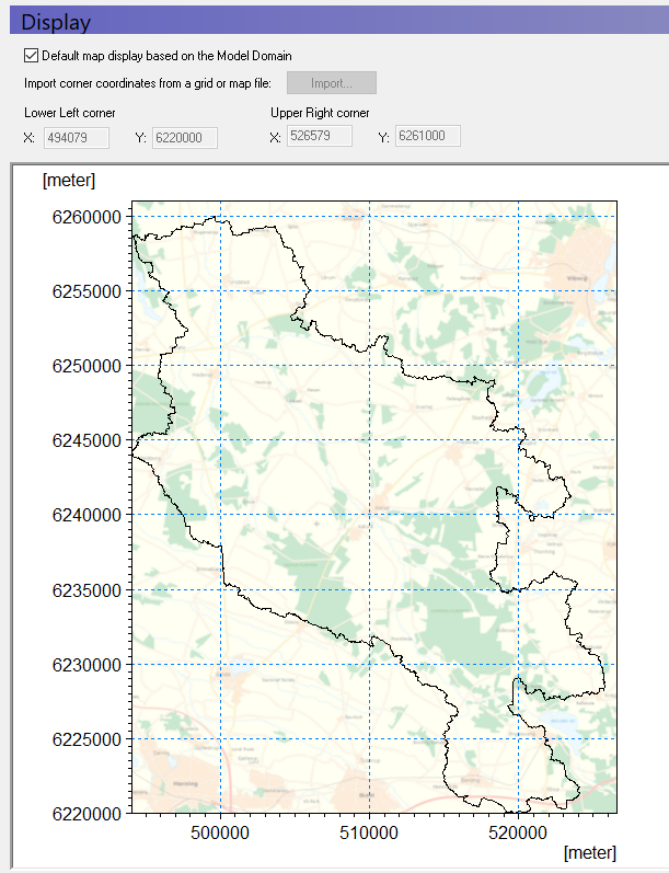
The option 'Default map display based on the Model Domain' means that the map view will be defined by the size of the model domain that you select in the next section of this exercise.

However, in some cases you may want the displayed map area should be much larger than the model domain, in which case you can define the map extents in this Dialog.

You can also import the extents from a shape or dfs2 file.

In this case choose the setting Default map display based on Model Domain.

This is how it will look once you have defined your model domain, further on in this exercise.

Add overlays

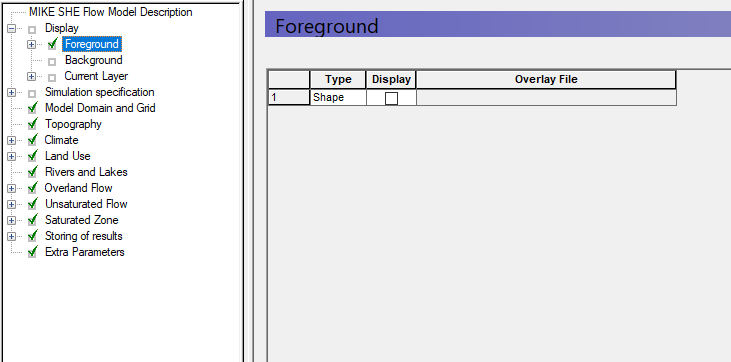
Two overlays will be added: A shape overlay showing the catchment and an image overlay showing a map of the area. In the Foreground Dialog under Display:

Click on the Add Item icon

Choose the type “Shape”

Add another item, but now choose “Image”

Notice that a plus sign (+) appears beside the Foreground item in the data tree. This indicates that sub-items have been added in the data tree.

The Background and Foreground options refer to the way the overlays are displayed relative to the input data specified in the other Dialogs. Typically, you only need the Foreground display active.

Also, if you have multiple overlays, the order that they are listed defines the order in which they are displayed. Thus, you don't usually want a bitmap at the top of the list, since it would hide all of the lower overlays.

Define the shape file

Now click on the plus sign beside the Foreground item in the data tree to expand the data tree. Then click on the sub-item “Shape: Unknown” to display the sub-Dialog.

In the dialogue you can also

Choose line-colour

Increase the line thickness (e.g. 0.5 or 1 mm)

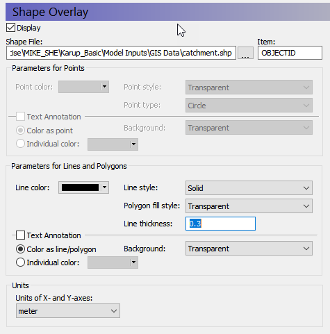
In the sub-Dialog:

click on the browse button

find the file
.\\Karup_Basic\\Model Inputs\\GIS Data\\catchment.shp

Define the image file

Now click on the subitem “Image: Unknown”. This shows you the following dialogue:

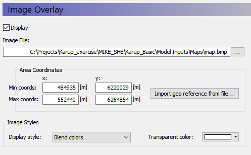
click on the browse button, , and find the file
.\\Karup_Basic\\Model Inputs\\Maps\\map.bmp

Since a bitmap image does not contain any geographical information (it is simply a list of pixel locations and colours), the bitmap must be oriented in space. To do so, you can either import the georeferenced coordinates from a world file or provide MIKE SHE with the coordinates of the lower left and upper right corners of the bitmap.

Type in the coordinates as shown in the figure above

Click on Display to make the map visible

Set the Display style as Blend Colors, which will blend the map colours with any other displayed colours. This will prevent the bitmap from hiding the model data.

Add more layers if desired. Line themes for showing the stream (karup_system.shp) are located in the same folder as the catchment file.

Note that these files will not be visible until you define your model domain, described further down. Once this is done, you should see the files in all of your map dialogues.

Set up the simulation

MIKE SHE includes several simulation modules. The navigation tree in the user interface depends on your choice of simulation modules.

Select simulation modules

In the Simulation Specification Dialog, make sure that all the Water Movement items are checked On. Make sure that:

Rivers and Lakes are on;

Finite Difference is selected for the OL and SZ engines, and

the Richards equation is selected for the UZ engine.

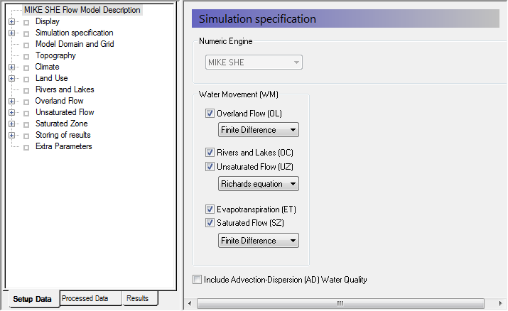
The Simulation Specification Dialog allows you to select which flow components to include in your simulation. For example, if you want to include only the river and the exchange to the saturated zone, then you only need to select Rivers and Lakes plus Saturated Flow.

Not selecting some of the items can be a useful option during the initial model setup stage when you are setting up and calibrating a complex model.

In this dialog, you chose the numeric engine for the different hydrologic processes.

There are three numeric engine options for the unsaturated zone and two each for both the Overland flow and Saturated Flow.

The calculation method for the Evapotranspiration is automatically selected depending on the Unsaturated Flow option selected.

The channel flow numerical method is selected in the MIKE+ Rivers Setup.

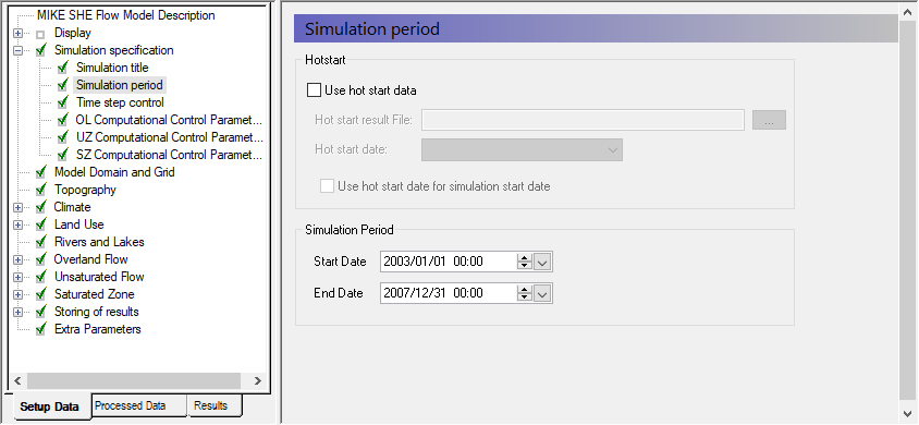
Specify the simulation period

In the Simulation period Dialog:

• Specify the Start date and End date
• Start Date: 1 January 2003

End Date: 31 December 2007

In this Dialog, you can either type in the dates or select the dates from a drop down calendar.

If your simulation runs too slowly, then you can reduce the length of the simulation period without affecting the learning objectives.

Specification of the simulation period at this early stage in the model development is not a requirement. However, it is convenient because the time-varying input data you specify later is validated against the simulation period. Thus, when you specify a rainfall time-series file, a check is made to make sure that the time-series covers the simulation period.

In most cases, MIKE SHE is run as a transient model. If the model is run in steady-state, then the steady-state solution also follows this simulation period, by generating a series of identical steady-state solutions for each specified time step.

Typically, you will start the simulation from a Hotstart condition. The Hotstart allows you to start the simulation from the end of a previous simulation. You will often create a ‘run-in’ simulation that allows the model to dynamically equilibrate. Then, start the actual simulation at, for example, the end of a dry season.

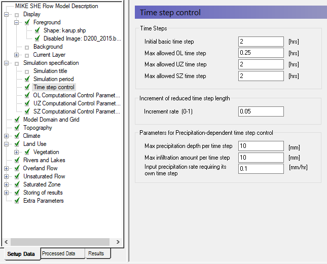
Define time step parameters

In the Time step control dialog specify:

Initial basic time step = 2 hrs

Max allowed OL time step = 0.25 hrs

Max allowed UZ time step = 2 hrs

Max allowed SZ time step = 2 hrs

Demo Note: If you are using a Demo version, you should use an SZ time step of 4 hours, as you will otherwise exceed the number of saturated zone time steps.

MIKE SHE uses different time-steps for the different hydrologic processes. Normally, the Overland flow time-step is the smallest and the Groundwater time-step the largest. The river time step is controlled in MIKE+.

The overland flow time step is quite small because it is highly dynamic. The overland time step has to be the same or larger than the MIKE+ Rivers time step.

Generally, the time steps are relatively small in this example because the system is quite sandy and highly dynamic. In a less dynamic simulation, you would normally make the SZ time step larger.

The Max infiltration amount and the Max precipitation depth per time step are used to improve the numeric stability of the solution when there is ponded water on the ground surface. If the maximum values are exceeded, then the time step will be automatically decreased until this limit is reached.

Simulation control

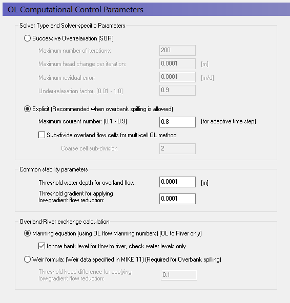
We will use the default values for all the solver parameters. Details on these parameters can be found in the on-line Help.

Overland flow

You should use the default parameters for OL, but change to the Explicit solver. Leave the Manning equation for calculating overland flow into the rivers.

If you want to calculate flooding, then the explicit solver is required. However, the time step constraints on the explicit solver are more restrictive.

Unsaturated flow

Change Maximum no. of iterations from 50 to 250. Keep the other default UZ solver parameters.

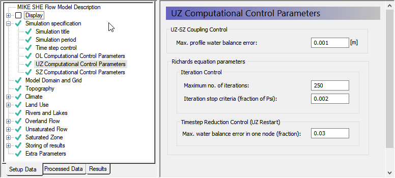
Richard’s equation for unsaturated flow may produce water balance errors if the time step is large and the control parameters are set too loosely. Increasing the iteration control parameters will however increase the runtime which may not be desirable.

Problems with the water balance are reported in the water movement run log file (stored in the Results folder) and should be checked at the end of every simulation. It is also advisable to run the water balance tool to make sure the model is performing correctly.

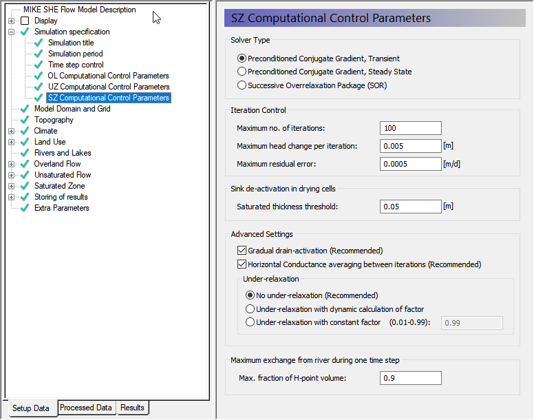
Saturated flow

You should use the default parameters for SZ including the default PCG Transient solver.

Change Maximum no. of iterations from 50 to 100. Keep the other default SZ solver parameters.

Set up the model domain

The model domain and the surface topography are required for all MIKE SHE components.

The model domain defines the horizontal extent of the model area, as well as the horizontal discretisation used in the model for overland flow, unsaturated flow and saturated groundwater flow

Define the model domain

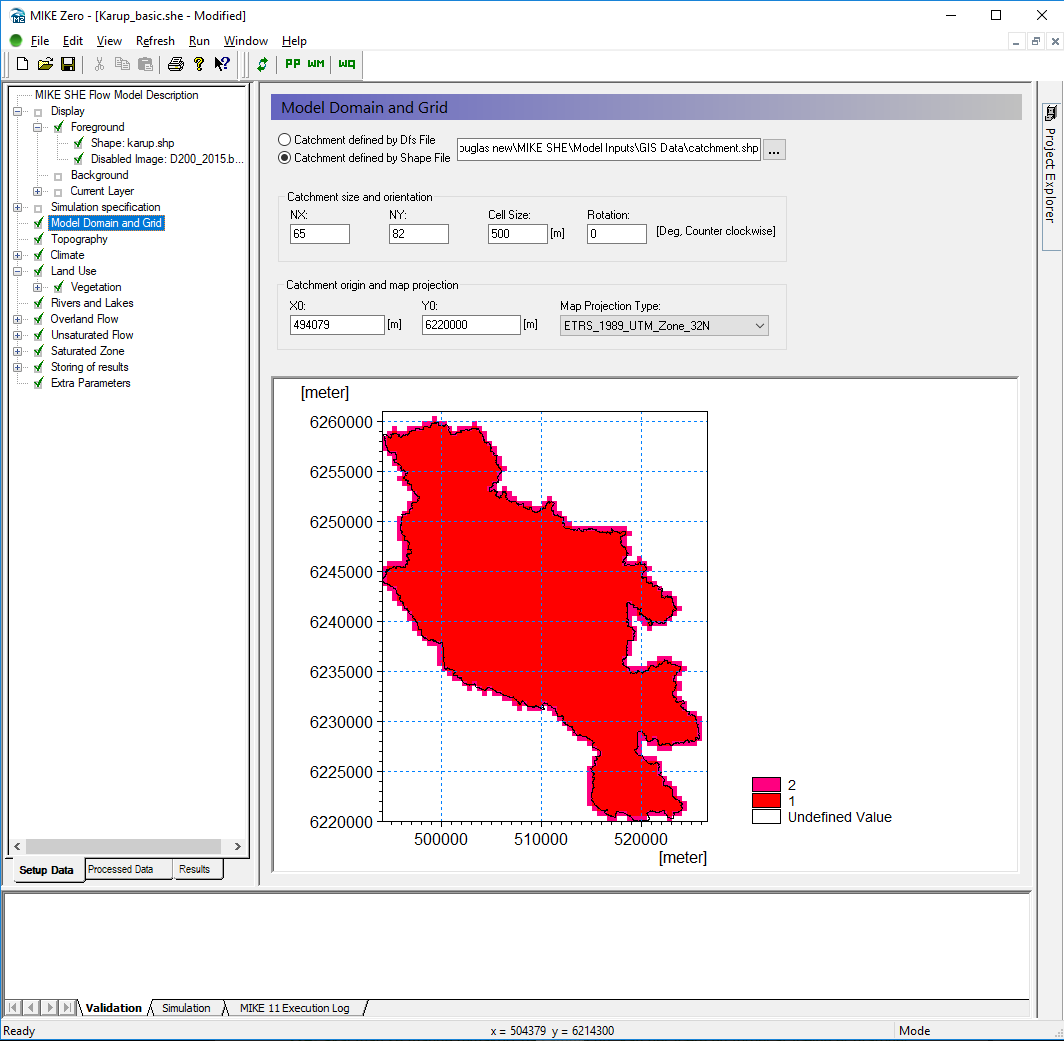
In the Model Domain and Grid Dialog:

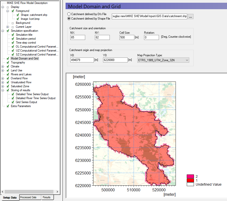
Choose Catchment defined by Shape File

Using the Browse icon, select the file .\\Model Inputs\\GIS Data\\catchment.shp

Set the Shape axis units to “meter” in the dialogue that pops up.

• Set the grid dimensions to
• Number of cells in the X direction, NX = 65
• Number of cells in the Y direction, NY = 82
• Cell size = 500m
• Rotation = 0
• Origin (X0, Y0) = 494079, 6220000

Demo note: If you are using a demo version of the software, you will not be able to have the same amount of cells. Instead use NX = 33, NY = 41, and Cell Size = 1000 m.

• Map Projection Type = ETRS_1989_UTM_Zone_32N

A list of previously used map projections will appear in the drop down menu when selecting Map Projection Type. To find and use the projection for the first time

click

go to: OpenGISProjections/Coordinate Systems/Projected Coordinate Systems/UTM/Other GCS/ETRS_1989_UTM_Zone_32N (or search for it using the Find… button on the right)

Click OK

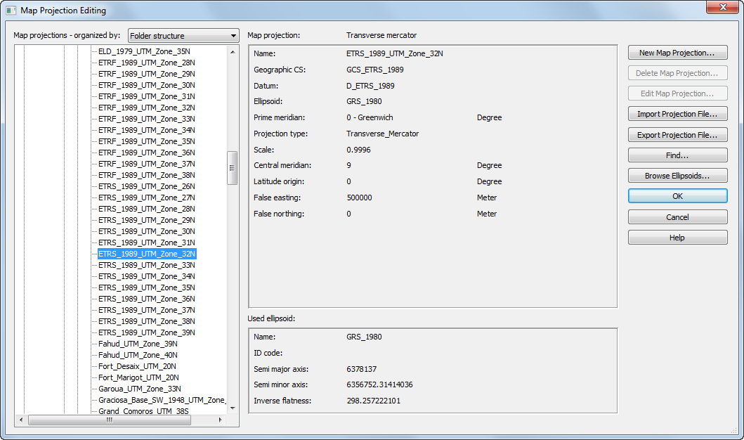
The Map Projection Type allows you to use any valid map projection. The only restriction is that whichever projection you chose, you must be consistent with respect to all other map inputs. You cannot mix, for example, maps from two different UTM zones.

The NON-UTM option implies local rectangular coordinates, without a map projection.

MIKE SHE automatically assigns values of 1 to the internal cells and values of 2 to the boundary cells.

When you preprocess the data, the preprocessor calculates the model domain based on the .shp file and defines the model domain as a dfs2-grid with integer values 1 (internal point), 2 (boundary point) and zero values for areas outside the model domain. The pre-processor assigns all of the model parameters based on the dfs2-grid that is calculated from the polygon that you have specified in this step.

If you wish to change the model domain, all you have to do is modify the .shp file and pre-process the data again. However, be aware that previously specified data must still cover the new polygon. If it does not, then either a warning will be issued (saying that some values were automatically interpolated) or an error will be issued (if it can't interpolate the data).

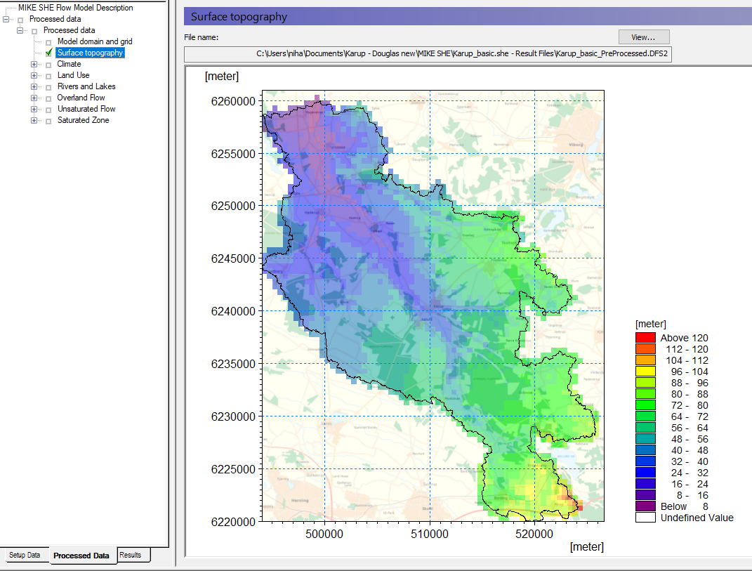
Set up the topography

The surface topography is required for all MIKE SHE components. The model topography defines the upper bound of the groundwater model as well as the upper surface of the unsaturated zone model. It is also used as the flow surface for overland flow.

Globally, Digital Elevation Model (DEM) data is widely available. Free DEM data at 90m and 30m resolution is available from the NASA SRTM data. There are also commercial providers of higher resolution DEM data, including DHI.

For Denmark, DEM data at different resolutions (0.4m, 1.6m and 10m) are available (https://dataforsyningen.dk). Data is provided as raster grid data in ArcGIS or MapInfo format. For this model, the 10m-resolution DEM data was downloaded and resampled to 50m. The data was then converted to a point ArcGIS shapefile.

The resampling can be important. High resolution DEM data will be interpolated in MIKE SHE. However, the GUI may become very slow if it is continually interpolating high-resolution data.

Define surface topography

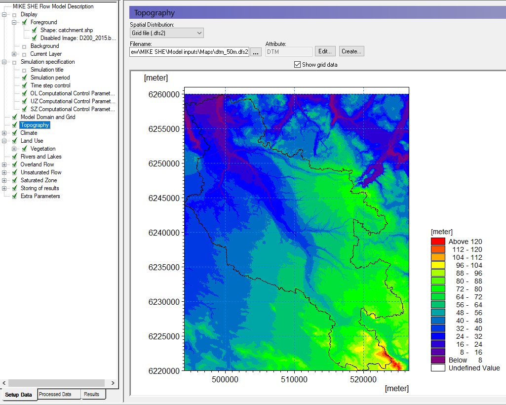
In the Topography Dialog:

Choose Grid file (.dfs2) for the Spatial Distribution

Select the file
.\\Model Inputs\\Maps\\dtm_50m.dfs2

Spatially distributed data, such as topography can be specified using:

• a Uniform value
• a Grid file (.dfs2),
• a Point/Line (.shp) ArcView or ArcGIS map, or

an ASCII file with distributed xyz values (Point XYZ (.txt)).

If a .shp file or a xyz-file is used, MIKE SHE will interpolate the data to the mesh defined in the Model Domain and Grid menu.

Hint: you can always see the Z-value at the cursor position at the bottom of your Graphical View.

Point/Line - Interpolation method - You can choose between Bilinear, Triangular, Inverse Distance and Inverse Distance Squared interpolation methods by selecting from the Interpolation method combo box.

• The Inverse distance methods are good for scattered data.
• Bilinear Interpolation is a good method for interpolating from gridded data and the
• Triangular method is good for interpolating from digitised contour lines.
• You can use the Online Help to find out more information on the interpolation methods, by clicking F1. At the bottom of the Help page, are references to Related Items, which will take you to the detailed descriptions of the interpolation methods.

SURFER - If you want to use interpolation methods not available in MIKE SHE, then you can use a program such as SURFER by Golden Software. In SURFER, you can save the interpolated SURFER grid to an XYZ file, and use the bilinear method in MIKE SHE to reproduce the Surfer interpolation.

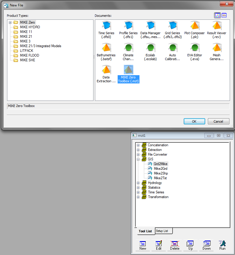
ArcGIS Grid – If you have gridded data from ArcGIS, then you can use the Grd2Mike Tool (New File\MIKE ZERO\MIKE Zero Toolbox\GIS) to convert an ArcGIS grid to a dfs2 file.

Other tips:

The search radius should be sufficiently large to ensure that each grid gets a value. For this exercise 1000 m is sufficient. However, the minimum search radius is two times the cell size. Search radii below this will have no effect. In this data set, the data density is quite high, and changing the search radius will have no effect.

In some cases, such as when the grid is very large or the number of data points is large, then the interpolation can be time consuming. This can be a problem, since the grid is re-interpolated every time you enter the Dialog, as well as during the pre-processing step. To make the model more efficient, you can save the interpolation to a dfs2 file for use directly. To do this, right click on the map view and select save to dfs2 file.

After you have saved the dfs2 file, you can then use it instead of the .shp file. Note though, that the link to the original .shp data is not lost, but simply hidden from view. This allows you to return to the original data if you want to change the discretisation of the dfs2 file, for example, if you change the size and shape of the Model Domain and Grid.

If you have high-resolution DEM data, often the most efficient process is to use ArcGIS to interpolate the DEM data to the grid resolution that you want to use. At the same time, ensure that the point values are located at the model nodes. This will limit the amount of re-interpolation in the GUI and ensure that your model topography is exactly as you expect.

Define climate

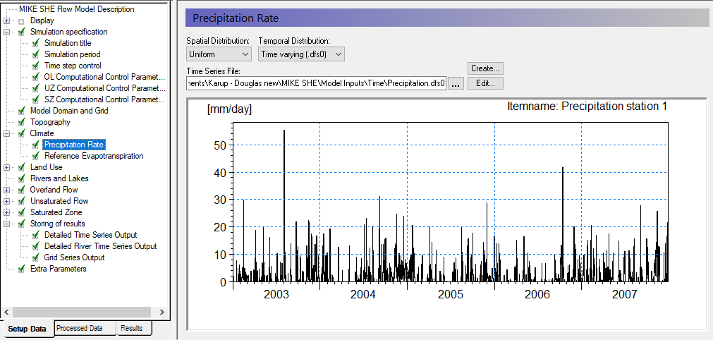
Define precipitation rate and temporal distribution

The precipitation is the actual amount of measured rainfall:

Go to Climate in the menu and select the sub-item Precipitation Rate

For now, choose Uniform Spatial Distribution, which means that the same precipitation rate will be used all over the model domain.

Change the temporal distribution from constant to time varying.

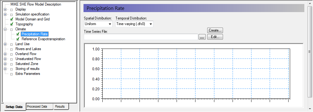
Click on the button to open the file browser

Navigate to .\\Model Inputs\\Time\\Precipitation.dfs0

Keep the default Item “Precipitation station 1” and click OK

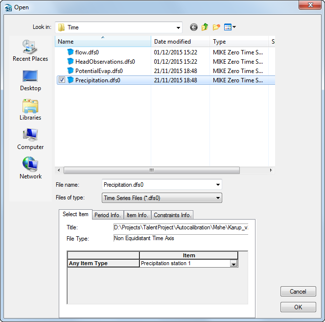
In this case, you are using spatially uniform recharge data. The precipitation file contains data from several rain gauges. The particular rain gauge to use is selected under the Item in the browse Dialog. In this case, you are using only the data from Precipitation station 1.

In this model we are using a uniform rainfall rate over the entire catchment. For small catchments this is reasonable. In large catchments this would not normally be correct. By selecting Station-based, we can define regions or Thiessen Polygons where different rain gauge data is used. If you have access to gridded rainfall data, for example from radar rainfall stations, then you can use fully distributed rainfall data as well.

Precipitation is specified the same way data is collected from rain gauges. It can be input as mean-step accumulated values (e.g. average rainfall per day in units of mm/day) or, as step accumulated values (e.g. measured rainfall in a tipping bucket rain gauge in units of mm since the last measurement).

Finally, your calibration will depend on the frequency of your rainfall data. Your model will react very differently if you have monthly rainfall averages versus hourly rainfall from a local gauge. If you update your rainfall frequency, you will normally have to recalibrate your model.

Add Reference Evapotranspiration

MIKE SHE calculates actual evapotranspiration based on the evapotranspiration rate, the vegetation properties, and the soil moisture.

In the Reference Evapotranspiration Dialog:

Use Uniform spatial distribution

Use Time-varying (.dfs0) Data Type

Use the browse button to select the file .\\Model Inputs\\Time\\PotentialEvap.dfs0

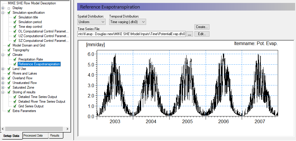
Reference evapotranspiration can be specified in the same manner as precipitation, that is, as constant or time-varying values and as uniform or spatially distributed values.

As you’re using Uniform distribution type, this evapotranspiration rate will be used throughout the model domain.

Evapotranspiration and Precipitation are highly correlated. Reference evapotranspiration is a function of solar radiation (sunshine), wind speed, relative humidity, and air temperature. All of these factors are affected by rainfall. Thus, it is desirable, but not critical, to use Precipitation and Evapotranspiration from the same weather station and at the same recorded frequency.

Add land use

Define the vegetation distribution

Under Land use select the Vegetation Dialog:

Use Station based Spatial distribution

Specify Grid Codes (dfs2) as the Data Type

Use the browse button to select the file .\\Model Inputs\\MAPS\\Landuse.dfs2

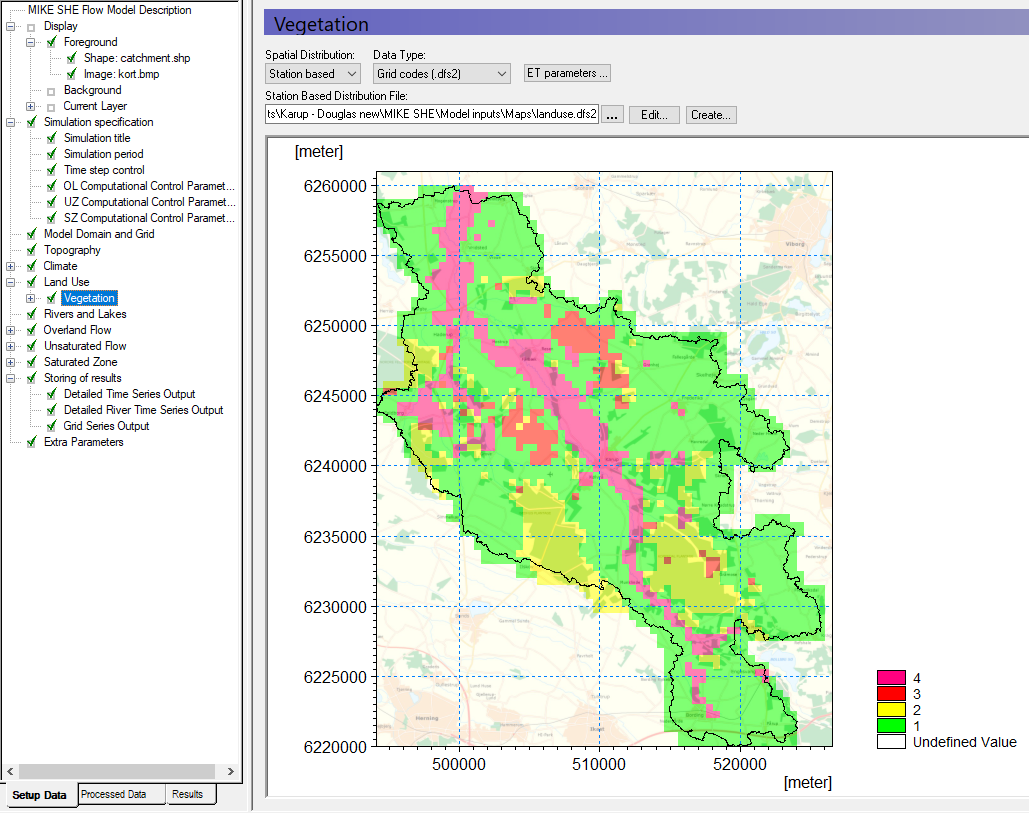
The map now displays your vegetation distribution. The map (dfs2 file) contains 4 different integer codes that define 4 different areas. You now need to define the vegetation types and growth function that are associated with the 4 different areas.

Define vegetation types for each vegetation area

Each of the 4 different vegetation areas in the vegetation map appears as a sub-item in the data tree.

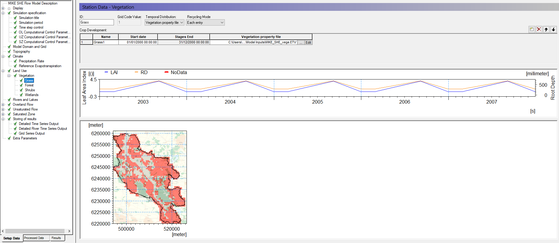
Select the Grid code = 1 item

Change the ID to Grass

Set the Temporal Distribution to Vegetation property file

Use the new items icon, , to add a line in the Crop Development table.

• On the line in the Crop Development table
• Use the browse button to select the vegetation property file (database file):
  .\\Model Inputs\\MIKE_SHE_vege.ETV
• BEFORE closing the dialog,

From the pull-down Veg type combo box pick Grass1

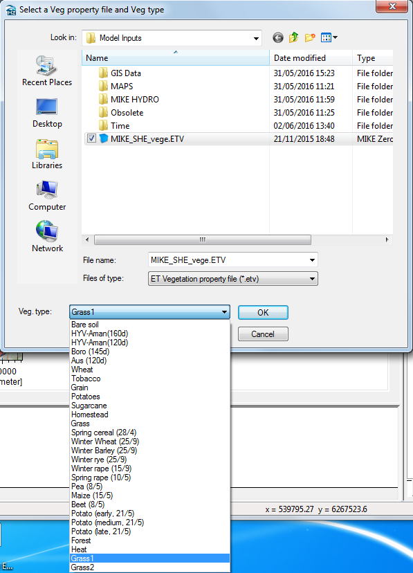
Set the Start date to 1. Jan. 2000

(The start date is set before the simulation start data to ensure a full coverage of the simulation period).

Set the Recycling Mode to Each Entry

For the remaining three vegetation types, set the Temporal Distribution to Constant and use the following values for the remaining items:

• Grid code = 2: ID=Forest, LAI = 6, RD = 800 [mm], Kc = 1
• Grid code = 3: ID=Shrubs,LAI = 2, RD = 500 [mm], Kc = 1

Grid code = 4: ID=Wetlands, LAI = 4, RD = 500 [mm], Kc = 1

LAI is the Leaf Area Index, which is a measure of the density of the vegetation in area of leaves per square area of ground [m2 leaves/m2 ground]. RD is the Root Depth.Kc is the Crop Coefficient which is effectively a scaling parameter on the Reference ET.

The Crop Development table allows you to define flexible crop rotation schedules.

The schedule is defined in the Vegetation database, and the Recycling Mode is used to define how the schedule is repeated during the simulation.

The recycling mode defines what happens when the crop rotation ends.

• If no recycling is defined, then the vegetation properties will revert to 0.
• Each Entry means that each line in the table is repeated until the next start date.
• Entire scheme means that the rotation table starts over again after the last entry.

Entries, then scheme means that the lines are repeated to fill in any gaps, and then the entire scheme is repeated.

For example,

• If you have one crop per year, then you can set up a simple annual schedule in the Vegetation database. Then if you choose the Each Entry option, the crop schedule will start over again as soon as it is finished. This is what we have done here.

If you have multiple different crops per year, or a fallow crop in alternating years, then you could set this up as multiple lines in the Crop Development Table, with two different vegetation types and schedules.

Note

The recycling does not account for leap years. So, if you have very long simulations that require precise crop rotation dates, then you may want to set up a 4 year cycle in the Vegetation database.

Add the river module

You will now add an existing MIKE+ Rivers setup to the model. Setting up the river in MIKE+ is detailed as a separate exercise in Section 5.

Add the river module

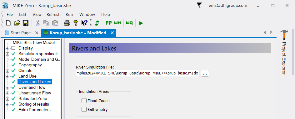
In the Rivers and Lakes Dialog:

• Use the browse button to select the existing .m1dx file (previously exported from MIKE+) for the Karup catchment:

.\\Karup_MIKE+\\Karup_basic.m1dx

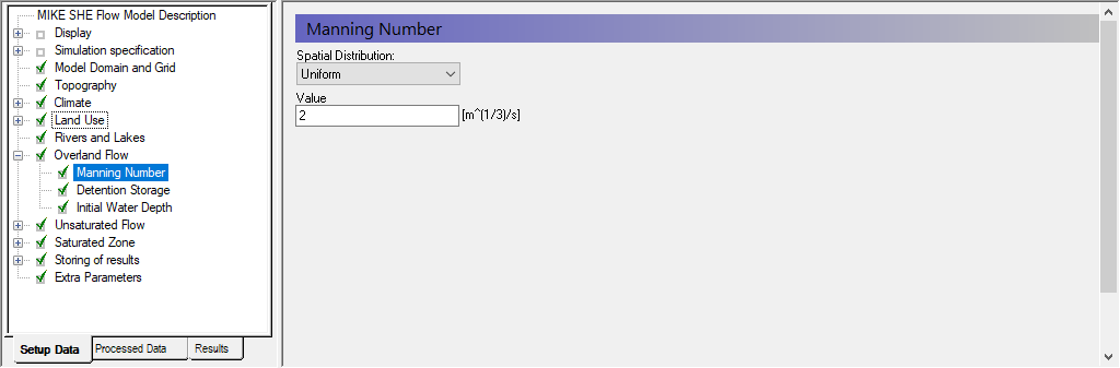
Specify the overland flow parameters

In the sub-items in the Overland Flow Dialog (in the MIKE SHE GUI), specify

Manning’s M equal to 2 [m1/3/s]

Detention storage equal to 4 [mm], and

Initial water depth equal to 0 [m].

The Karup catchment is quite sandy, and in this simulation there are no serious storm events. Thus, in reality, overland flow is insignificant for this simulation.

The detention storage cuts off overland flow when the depth of ponding is less than the Detention storage. In this case here, all rainfall events below 4mm will not generate overland flow directly.

You can disable overland flow by specifying a Manning’s M = 0 [m1/3/s]. Setting the Manning’s M to zero locally is sometimes a useful way of speeding up the simulation by turning off the overland flow calculation in areas of permanently ponded water, such as small reservoirs. However, a Manning’s M of zero will prevent any overland flow from entering the cell.

The Detention Storage defines the depth of ponding required before Overland Flow occurs. A high Detention Storage value will effectively turn off Overland Flow. Again, this is very useful when you want to locally turn off Overland Flow, for example in lakes or ponds.

You can play with the Overland flow parameters later, if you like. For now use the value stated above.

Build the unsaturated zone model

The unsaturated zone model calculates recharge to the groundwater model and is closely linked to the actual evapotranspiration, as the roots remove water from the unsaturated zone. Soil physical properties are stored in a soil-database. The link between soil-type distribution maps and soils in the soil-database are established similarly to the link between vegetation-distribution maps and vegetation types.

Calculation column classification

In the Unsaturated Flow Dialog use the default values.

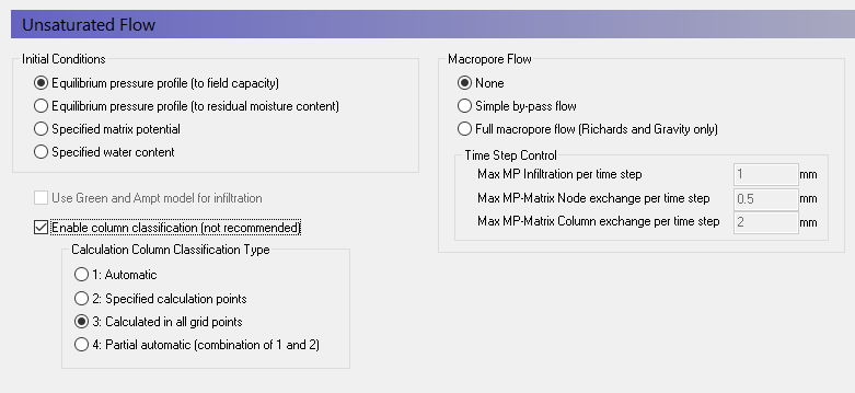
When using Richards Equation or Gravity Flow, the default initial condition for UZ is an equilibrium pressure profile based on the saturation-pressure curve. However, there are two options. In temperate areas, the soil moisture below the root zone is typically close to field capacity. However, in arid areas, the moisture content below the root zone can be much drier. Thus, there are two options for the initial UZ soil moisture where the minimum initial water content is 1) field capacity or 2) the residual water content.

You should avoid Automatic UZ column classification and always use Calculated in all grid points (default).

MIKE SHE allows you to lump similar UZ profiles together to reduce the computation time. In this case, the results of one column are copied to other similar columns. This option was very useful in the past when computers were slower. However, this should be avoided now. The option has been retained to support backwards compatibility and some special cases.

Demo Note: You must use the Automatic Classification if you are using the demo version. In the Demo mode, the model size is restricted to a maximum of 155 UZ computational cells

Define the soil profile distribution map

In the Soil Profile Definitions Dialog:

Use Distributed for the Spatial Distribution

Use Grid codes (dfs2) distribution data type

Use the browse button to select the dfs2 grid file .\\Model Inputs\\Maps\\soil.dfs2

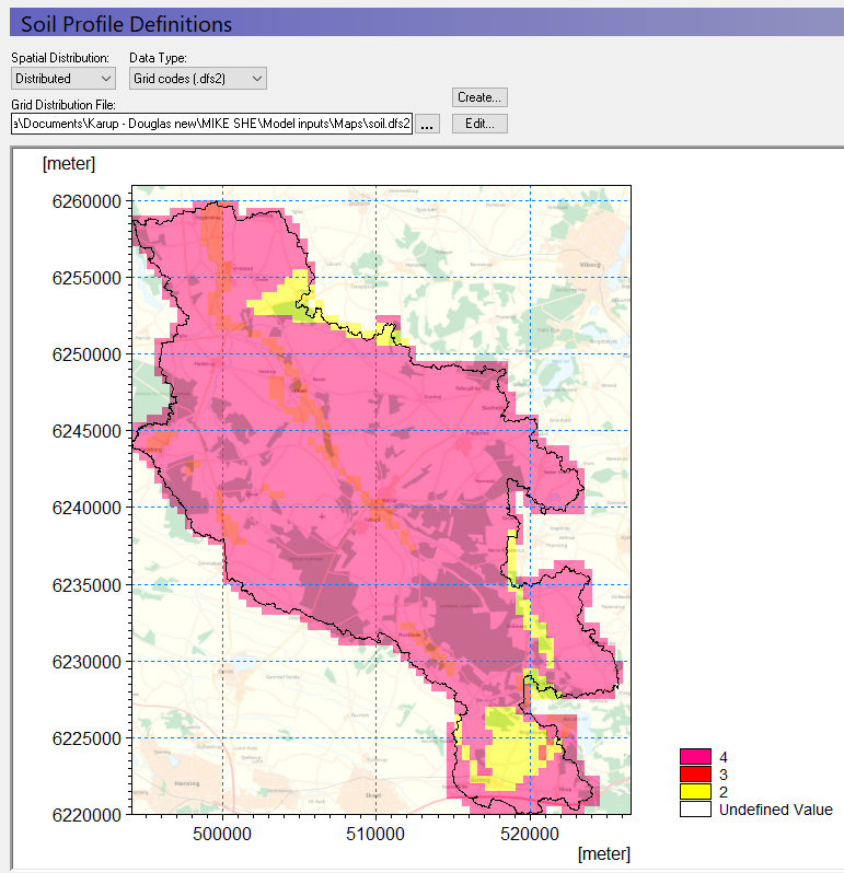
The soil map contains three different code values, which now need to be associated with three soil profiles.

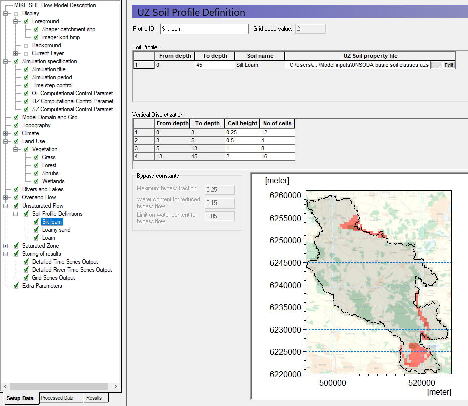
Define soil profiles (horizons)

Each of the 3 different soil areas in the soil map appears as a sub-item in the data tree. For each soil zone

Select the line in the Data Tree (Grid code 1, 2, etc)

Set the Soil Profile depth to 45 m

Use the browse button to select the UZ soil-database file .\\Model Inputs\\UNSODA basic soil classes.uzs

BEFORE clicking OK, select the soil type as follows:

Grid Code = 2	Silt Loam
Grid Code = 3	Loamy Sand
Grid Code = 4	Loam

• Rename the Profile ID

Add 4 lines to the vertical discretization, using the add button

Set the vertical discretization as follows:

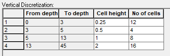
To facilitate the process you can add four lines using the add button . Then select all the lines in the table (click in the upper right corner of the table). Then copy and paste the vertical discretization table into the other soil zones.

The UNSODA database is a list of standard soil types developed by the US Department of Agriculture.

We are ignoring Bypass Flow in this exercise because of the sandy nature of the soils. You can use Bypass flow to account for variable flow rates in a soil column due to heterogeneities in the soil.

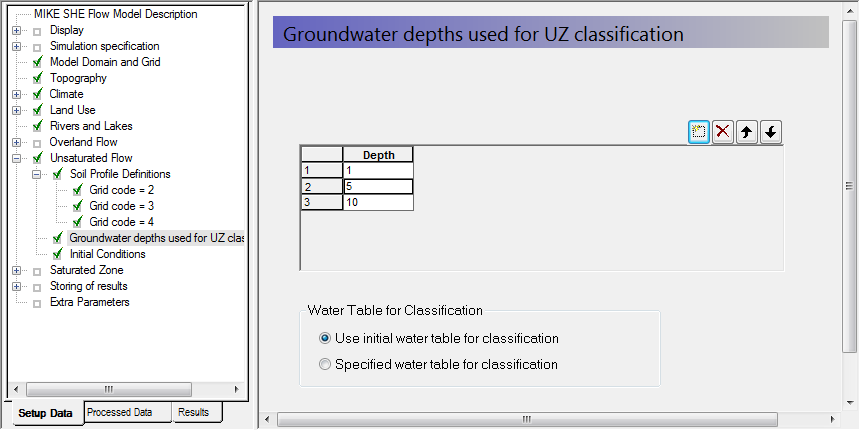
Demo Note: If you are using the Demo mode, then you must use the Automatic classification method, which requires you to specify a water table

The depth to the groundwater table is one of the criteria that are used when the automatic (lumped) unsaturated zone classification is used.

• In the Unsaturated Flow dialog change the Classification Type to 1: Automatic
• In the Groundwater depths used for UZ classification dialog specify Use initial water table for classification
• Define 3 depth classes 1, 5 and 10 meters

Build the saturated zone model

Before defining your computational layers you must input a geological model, which is defined as part of the saturated zone.

A geological model may be defined as a combination of layers and lenses. Once the geological model is defined you may choose computational layers that are either identical to the geological layers or you may choose different computational layers. If the computational layers differ from the geological layers MIKE SHE’s pre-processor will transfer the hydraulic properties of the geological model to the computational mesh.

Specify the Saturated zone (groundwater) options

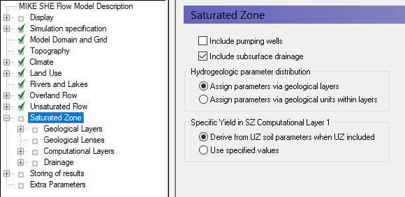
In the Saturated Zone dialog:

• Select Include subsurface drainage. This will ensure that any springs drain to the streams.
• There are no pumping wells for now, so make sure that the Include pumping wells is not selected.

Select Assign parameters via geological layers

The geology data can be assigned using both geological layers and geological units. If you choose the geological layers approach then the hydraulic properties are assigned as spatially distributed within the layer. If you use gridded data or point data, the hydraulic properties are smoothly interpolated to the model grid.

If you chose the geological units approach, then you must specify a distribution of geological units for each geological layer, for example, by a polygon file. In this case, all of the model cells in each polygon are assigned a value for each of the hydraulic properties.

The geologic units method is often specified when you use the AUTOCAL program for parameter estimation and automatic calibration. In this case, the parameters for each polygon can be estimated automatically and the model sensitivity for each parameter calculated.

By default the Specific Yield is derived from the UZ soil properties. The Specific Yield is calculated as (UZ Saturated Water Content) – (UZ Field Capacity). This ensures that the fluctuations in the water table will be consistent between the UZ and SZ models.

Define the number of geologic layers

In this exercise, we will only have one numerical layer.

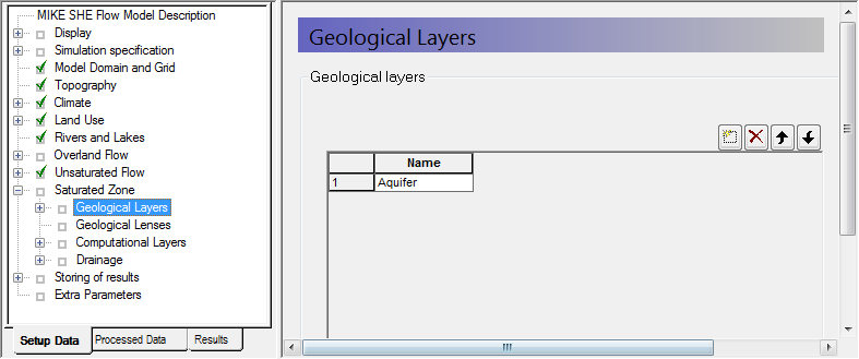
In the Geological Layers dialog:

Keep the existing default layer name Aquifer

By default there is already one layer in the model. Additional layers can be added by clicking on the Add Item icon, , deleted by clicking on the Delete Item icon, , or moved up and down by clicking on one of the Move Item icons,

Each of the Geological layers includes one item in the data tree for each of the properties. Additional layers will add additional sets of items to the data tree.

Increasing the number of saturated zone model layers allows you to better represent vertical flow and exchange between geologic layers. A fine vertical discretisation may also be required for solute transport simulations.

MIKE SHE allows you to have any number of layers in the saturated zone. However, the more model layers you have, the higher the computational effort and the more memory is needed. If you need more layers, it is always better to start with a few layers and do the initial calibration. Then add layers as necessary, while ensuring that the model remains stable and computational effort remains reasonable.

Define layer bottom (lower level)

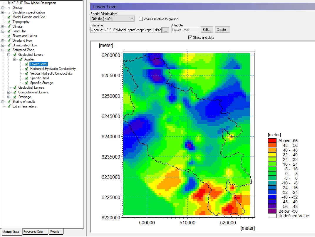
In the Lower Level Dialog for Aquifer:

Select Grid file (.dfs2) in the Spatial Distribution combo box

Using the file browse button, , select the file
.\\Model Inputs\\Maps\\layer1.dfs2

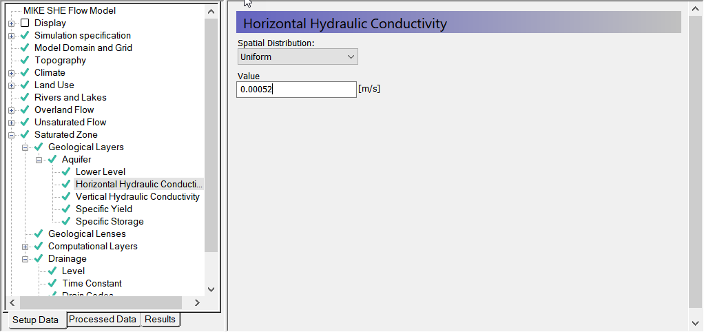
Assign hydraulic properties

The remaining hydraulic properties are listed under the Lower Level item. For each item:

• Select Uniform under the Spatial distribution combo box and specify the following values:
• Horizontal hydraulic conductivity = 0.00052 [m/s]
• Vertical Hydraulic Conductivity = 9.3e-5 [m/s]
• Specific Yield = 0.2 [-]
• Specific Storage = 0.0001 [1/m]

Define attributes of groundwater computational layers

The computational layers are defined independently of the geological layers. While the Geological Layers have geological attributes, the Computational Layers include computational attributes such as initial conditions and boundary conditions. The properties of the geological layers are mapped and interpolated to the computational layers during the model preprocessing.

Although MIKE SHE allows you to define Computational Layers independent of your Geological Layers, in this exercise computational and geological layers will be identical.

In the Computational Layers Dialog:

Select Defined by geological layers as the Type of Numerical Vertical Discretization

Use Minimum layer thickness = 0.5 [m]

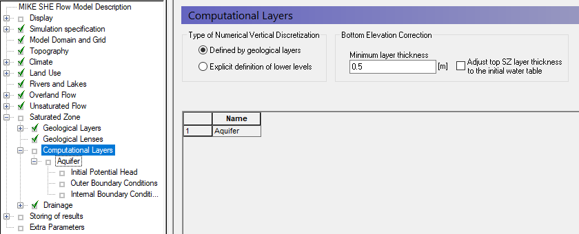
The Bottom Elevation Correction is used when you have multiple computational layers. In the exercise here, neither are relevant because we have only one SZ layer.

The Minimum layer thickness is used to keep layers from crossing or completely pinching out, which would cause numerical difficulties.

We recommend that you discretize the top of the SZ model such that the water table is always in the upper SZ layer. This ensures that the UZ model takes care of vertical UZ flow and the SZ model takes care of the lateral flow at the water table. To make this easier to manage, there is an option to adjust the upper SZ layer to be consistent with the initial water table that you defined. In this case, the upper SZ layer will be pushed down to the initial water table (minus the minimum layer thickness).

Define groundwater initial conditions

In the Initial Potential Head Dialog:

Select Grid file (.dfs2) under Spatial Distribution

Using the file browse button, , select the file
.\\Model Inputs\\Maps\\init-head-500.dfs2

Make sure that the Values relative to ground is turned off.

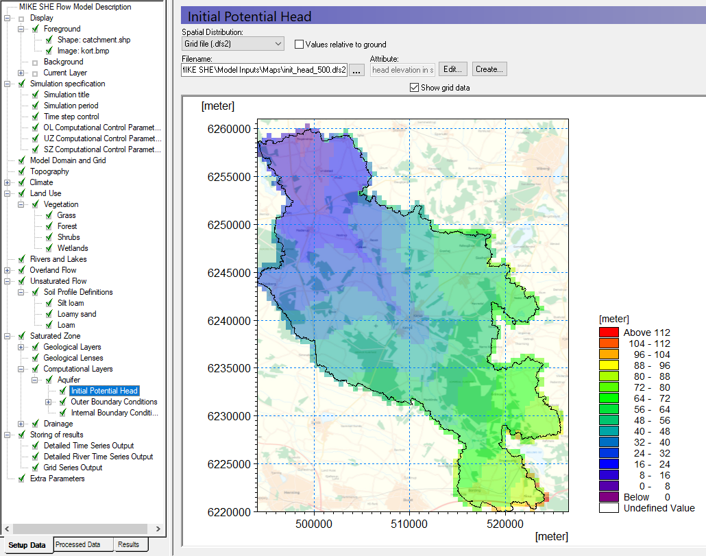
You are using an initial head from a previous model run, which gives you a good starting point. In a real model, you might initially start from a value such as 3 m below the topography. However, such a value will require a “run in time”, as the model may take several months to equilibrate.

Demo Note: In the Demo version, you need to run with a different grid size. To ensure that there is data in all grid cells, choose the file init_head_1000.dfs0 instead. It is located together with the file used above.

However, in most cases it is more effective to use a Hot Start. If you use a Hot Start, then the initial condition defined here is ignored, even though it must still be included.

An alternative is to run the model as a steady-state simulation and then use the steady-state solution as an initial condition. However, the steady state solution still might not be a reasonable starting point depending on how steady the groundwater table is. For example, the steady-state condition with pumping active might, in fact be nearly dry.

Define groundwater boundary conditions

The Outer Boundary is defined by the row of cells on the outside of the model domain. The outer boundary is defined by the Model domain and grid file, as all points with a code value of 2 (boundary point).

In the Outer Boundary Dialog:

Press the Add Item Icon,

Select Zero Flux (default) as the boundary type

Click on the Add Point icon, , and click anywhere on the map

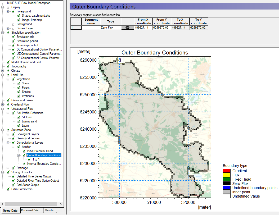
This now gives you a no-flow boundary condition along the entire outside of the model. If the entire outer boundary is a no flow boundary, then this step is actually unnecessary because by default the outer boundary is no flow.

The outside of the model can be divided into boundary sections, by clicking on the Add Item icon again. Then click on the Add Point icon, , again. Finally, click on the map to define the location of the boundary end point. The boundaries are specified clockwise around the model starting at the first point in the table.

The outer boundary conditions are defined independent of the model grid. Thus, if you change your model grid the boundaries will be interpolated automatically to the new grid based on the nearest boundary cells to the point locations. If you change the shape or extent of the grid, you should check that your boundaries have not moved unexpectedly.

Internal boundaries are used to specify such things as lakes and reservoirs that are not included in MIKE+ Rivers. In this case you could specify a constant head or a general head boundary for a lake.

Internal boundaries are distinguished from outer boundaries because on the outside of the model, you can specify flux and gradient boundaries.

Define the subsurface drain reference system

Under Drainage, choose Drainage routing based on grid codes

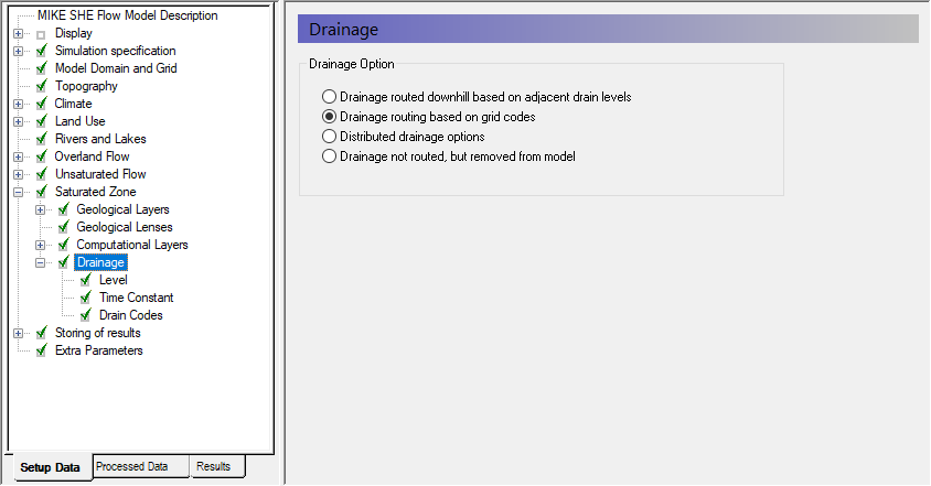
Drainage routing can be a very complex process. Simply removing the water from the model is the simplest drainage option. However, in most situations, drainage actually discharges to the river system.

Groundwater Drainage is a very powerful feature of MIKE SHE.

• The simplest routing method for the drainage is to route it downhill based on the drain levels. The drainage will enter the river whenever it intersects a river link. However, this can lead to ponding in local depressions in flat terrains, or inconsistencies in the drainage directions if the topopgraphy is not hydrologically correct.
• More complicated is the second option Drainage routing based on grid codes, where the drainage is routed downhill but only from certain cells. However, if you specify a single Drain Code, then the drainage will be to the nearest river.
• The Distributed drainage options allow you to route drainage to specific MIKE+ Rivers computational points or MIKE+ sewer manholes.

Define groundwater drainage

In the Drainage Level Dialog:

Select Uniform under Spatial Distribution

Use the value : -0.5 [m] (Note negative sign)

Check on “Values relative to ground”

The Values relative to ground tells MIKE SHE that you have drains located 0.5 meter below ground surface in the entire model domain. In this model, if the groundwater table is less than 50cm below the topography, groundwater will drain to the nearest river.

In the Time Constant Dialog:

Select Uniform under Spatial Distribution

Use the value = 5.6e-008 [1/s]

The drain time constant can be thought of as an empirical factor that accounts for the time it takes for the water to drain. For example, in the case of agricultural drains, the time constant could be affected by drain spacing, drain diameter, clogging, etc. In the case of natural drainage, the time constant is affected by the distribution of drainage ditches and channels.

A time constant closer to 1 implies that the water drains more quickly and the drain acts more like a constant head boundary, when the water table is above the drain level. Whereas, a value closer to 0 implies that the water drains more slowly. A value of 0 turns off the drainage.

You can define time-varying drainage parameters if you use a time-varying dfs2 file.

In the Drain Codes Dialog

Select Uniform under Spatial Distribution

Set the Grid Code value = 1

A single drain code will drain all groundwater drainage to the nearest river node.

Specify output options and calibration targets

In MIKE SHE, there are 3 primary outputs:

Detailed WM time series – This is a point value of a MIKE SHE output at EVERY time step, for example, Depth of Ponding.

Gridded output – This is a 2D or 3D grid of values of a MIKE SHE output at every STORED time step, for example groundwater head elevation.

Detailed river time series – This is a point value of the water level or flow rate in the defined streams in the model.

Both Detailed Time Series Output types automatically generate an HTML plot of the value as the simulation progresses. It also allows simulated output to be compared to observed output and calculates a number of statistics for model error. The HTML plots can be copied directly into reports.

The Gridded output is stored less frequently to conserve space on your hard disk. Likewise, many gridded outputs are not saved by default. Gridded output is stored as dfs2 (2D grid time-series files) or dfs3 (3D grid time-series files). If output data is stored too frequently, you may get very large and unwieldy result files. Thus, before running the simulation you should consider what and how often you need to save the data

A time series can be created for any point in the model domain from the Gridded Output, but the frequency of the values will be the same as the Storing Timestep. .

More detail on evalutating the output is in the next step-by-step Exercise.

Storing of results

Click on Storing of Water balance data

Set the Storing interval for grid series output to a daily frequency (24 hours) for Overland, Prec(ipitation) ET UZ, SZ-heads and SZ-fluxes.

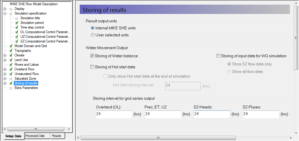
The Water balance items are used during the post-processing of the results to calculate water exchanges between the various components

The Hot start data is used for starting simulation from a previous result. This is useful when the run-in time for the simulation is long. In this case, you can run the initial simulation for a year or two. Then start subsequent simulations from a more reasonable initial condition. A good rule of thumb is to use a hot start condtion near the end of the dry season, when water levels are low and conditions are more stable.

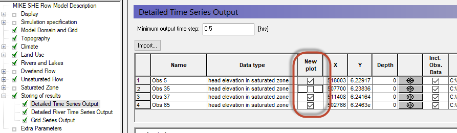
Define detailed time series output items

Select the Detailed WM timeseries output

Use the Add item icon, , to add 4 items to the list

• For each item,
• Set the name
• Select head elevation in saturated zone under Data Type

Define the X, Y coordinates from the table below:

Name	X-coordinate	Y-coordinate
Obs 5	518003	6229169
Obs 35	507700	6238357
Obs 37	511408	6241637
Obs 65	502766	6246299

Define the Depth = 5

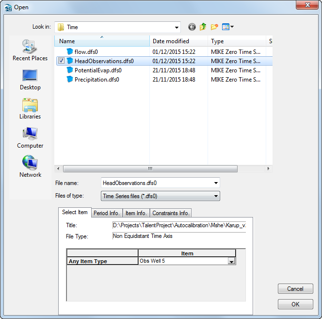
To add the observation data, you need to

Check on the Incl. Obs. Data checkbox

• For each observation point,

Use the browse button to select the file .\\Model Inputs\\Time\\HeadObservations.dfs0

• BEFORE clicking OK, you need to select the appropriate Item from the combo box. (e.g. Obs well 5 for the entry named Obs 5)

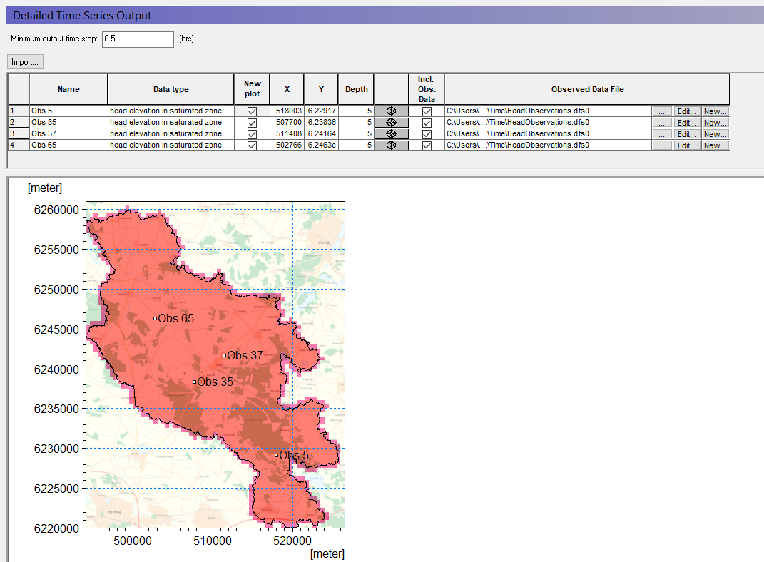
The X and Y location can be selected on the map using the button. This is useful if you want to create a detailed output of specific output items at a critical locations.

You are also welcome to add any other points and data items you like.

The New Plot checkbox is used to define whether or not a new html plot is created during the simulation. For example, if you uncheck the first box, then the first two items will be plotted on the same graph.

Create a detailed time series for the MIKE+ Rivers output

MIKE View is used to evaluate the output from MIKE+ Rivers. However, MIKE SHE allows you to create a detailed time series with observations during the simulation, similar to the other MIKE SHE outputs.

Add a detailed discharge time series to the end of the Karup River.

Under Storing of results select Detailed River timeseries output

Specify the name and location below:

• Name: 20.05 (outlet)
• Data type: Discharge
• Branch name: Karup River
• Chainage: 70454
• Incl Obs: check
• File name: .\\Model Inputs\\Time\\flow.dfs0, and then select the item: 20.05

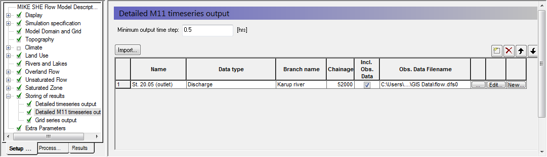
To add a Detailed MIKE+ Rivers time series, you have to know the chainage of the h-point (for Water Level) or the q-point (for Discharge) ahead of time. If the value is not exact, then MIKE SHE will look for the nearest point, within a certain search radius. If the nearest point is outside the radius, the pre-processor will print a warning, but still use the point. If there is no nearby point, then the output will be moved to the nearest point.

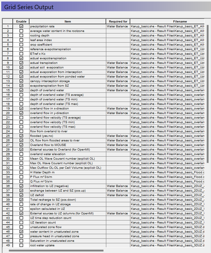
Select gridded outputs

In the Grid series output Dialog many items will already be selected if you have turned on the storing of Water Balance data.

• Some gridded items of interest are not connected to the water balance data. By clicking on the check box, turn on
• 1. Actual evapotranspiration,
• 1. Total Recharge to SZ, (pos. down)
• 1. Water content in the unsaturated zone.and
• 1. Depth to top phreatic surface (negative)

Running and evaluating MIKE SHE Flow Model

You can start this exercise by either loading a pre-defined MIKE SHE setup file, or using the model that you developed in the previous chapter.

If you are starting the exercises here, then

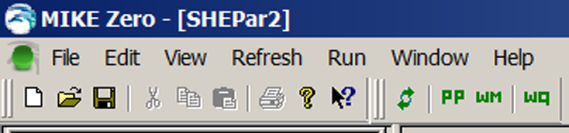
• Use the Open icon to open the Karup_basic.she file

This model should be similar to the model you would have obtained by following the step-by-step instructions in the previous Chapter.

If you are continuing this exercise from previous section,

• Open your MIKE SHE model setup that has been defined with the filename as e.g. Karup_basic1.she or MyFirstMSHE.she.

This exercise will familiarize you with the various output functions in MIKE SHE. However, the exercise will guide you through only the most basic functionality of the tools, including the Result Viewer, the Plot Composer, and the Water Balance tool

Pre-process the data

You have now specified all the input required for the model. Up to this point, all of the input data has been specified independently of the numerical model. You have specified only the characteristics of the numerical model that will be run.

Before actually running the model, you must run the Pre-Processor. The Pre-Processor extracts all of the spatial data that you have included and builds the actual model files.

Run the preprocessor

Click on the icon to start the Pre-Processor.

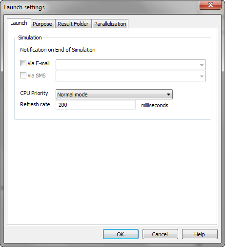
The preprocessor will start the MIKE Zero Launch utility.

• Click OK

Upon successful completion of the Pre-processing, you should check the model pre-processor log file to ensure the pre-processing finished without any errors. If the Pre-processing did fail, then the log file should contain some information to help you locate the problem.

The Pre-processed log files are by default located in the Result folder under MIKE SHE exercises.

Go to the results in Result\YourFilename.she - Result Files (e.g. Result\Karup_basic1.she.she - Result Files) folder and double click on YourFilename_PP_Print.log (the file should open in Textpad)

Scroll to the bottom of the file and check that the last line to ensure that the Pre-processing was successful.

View the preprocessed data

After successfully running the Preprocessor,

Click on the Processed Data Tab located at the bottom of the Navigation Tree.

• Then, click on the items in the data tree and explore the processed data.

The pre-processor creates a .fif file that contains the cell values etc. that will be used in the simulation. The processed data has been interpolated to the computational mesh, exactly as the simulation engine will read it. However, the .fif file is a binary format optimised for use by the numerical engine.

The .fif file embeds all geometric data. Temporal data (time-series data) are not contained in the .fif file, but are read directly from the source data files during the simulation.

To view the pre-processed data, a parallel set of .dfs2 and .dfs3 files are also created so that the standard MIKE Zero tools can be used to view the data.

It is the dfs data that is shown in the data tree and listed in the file name text box. Clicking on the View button opens the Grid Editor with the current pre-processed data file loaded – with all the current overlays.

Spend some time moving around in the Processed Data and make sure you understand the input data and the relation between Setup Data and Processed Data.

If you want to change any of the values in the Processed Data, you cannot just change the values in the Grid Editor. The values that you see are not the ones that will be used in the simulation. Therefore to change the values you have to:

• Edit the values in the Grid Editor,
• Save the parameter to a new dfs2 file, and

Then edit the Setup tab parameter to read from the new dfs2 file that you created.

View the river link setup

The MIKE+ Rivers network is interpolated to the cell boundaries of the model grid. The interpolated river locations are called river links.

In the Processed Data Tab the most recent pre-processed file is automatically loaded

• Go to the River Links Item in the data tree to view the pre-processed river links:

View the location of the river links in the computational mesh.

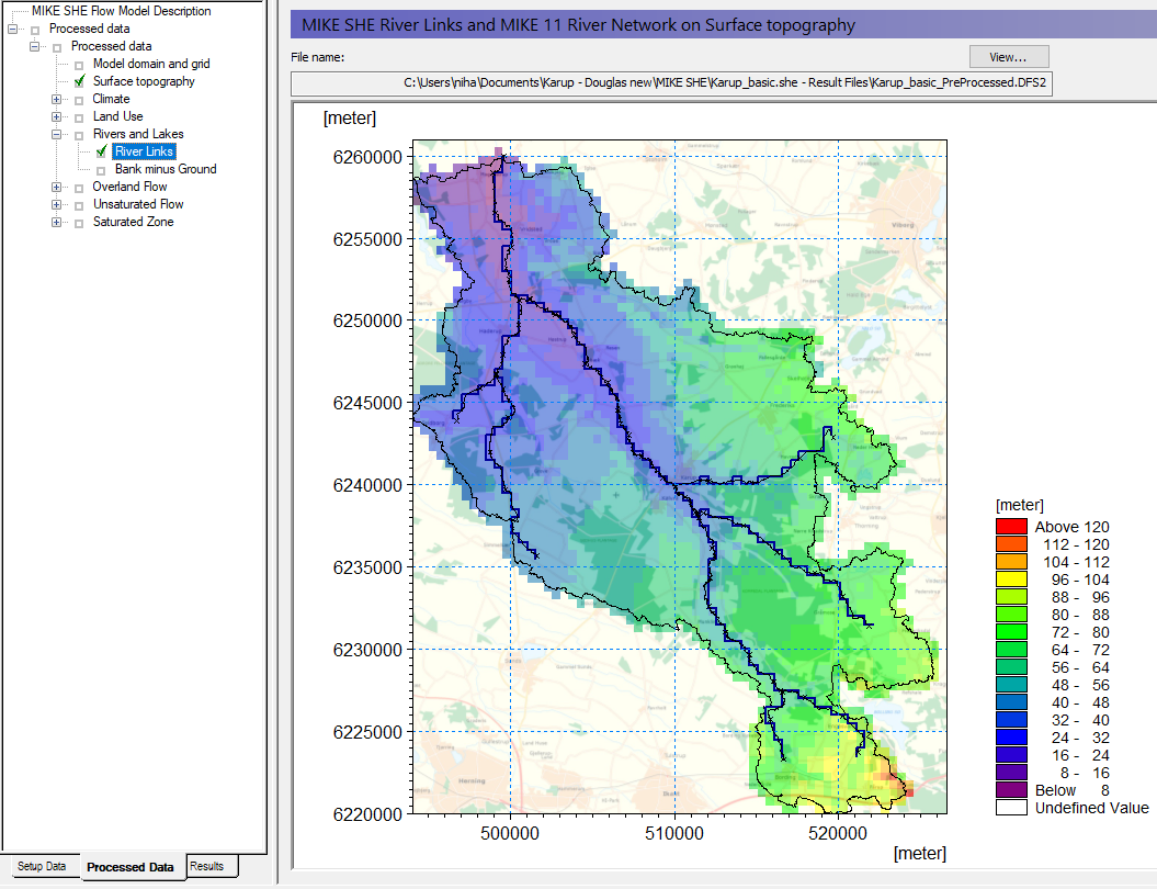
A .shp file of the River Links is also automatically created during the pre-processing. This file can be loaded as a background map in MIKE SHE, or in any of the MIKE Zero display tools, such as the Grid Editor, Plot Composer, and Results Viewer.

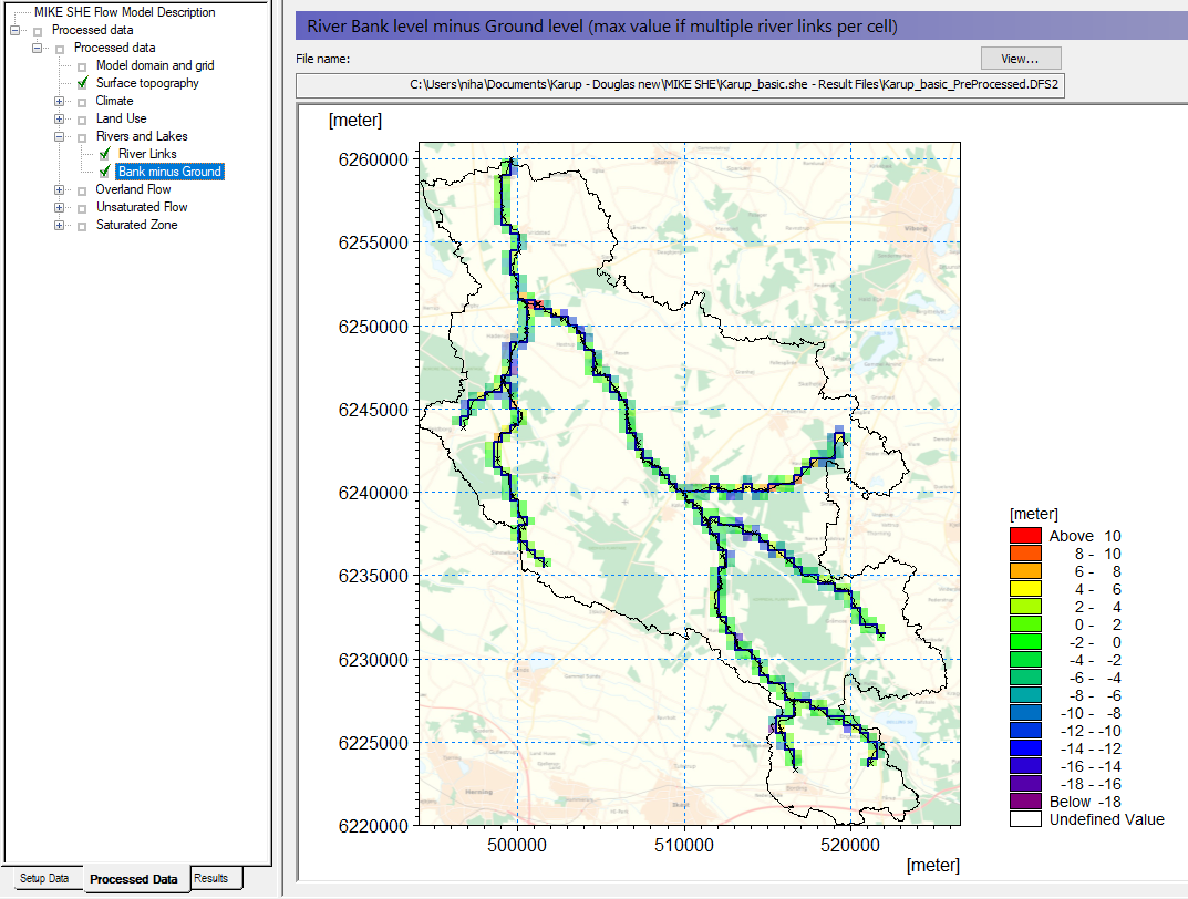
View the river bank elevations vs topography

A mismatch between the topography and the bank elevations will sometimes lead to poor OL-River exchange. You can use this item to locate areas were bank elevations are poorly matched to the topography. Occasional, random areas of mismatch are OK.

The cross-sections are specified in MIKE+. Each cross-section includes a left and right bank elevation. These elevations define how the river interacts with Overland flow.

In our model here, overland flow will flow into the river if the water level on the land surface is higher than the river level. Water will not spill out of the river.

However, if overbank spilling is allowed (Default = off), the river will spill on to the flood plain if the river water level is higher than the bank and higher than the topography. This requires the weir formula to be used in the OL Computational Control Parameters dialogue under Simulation Specifications. The bank levels act as weirs, and the water level must be higher than this “weir” to cross.

In the case where inflow to the river is restricted by the bank elevation, if water ponds along the edge of your river, it will normally infiltrate and enter the river via baseflow.

A poor match in the elevation is sometimes a sign that your cross-sections are much wider than your cell size. Typically, the elevation rises away from the river, and if you define cross sections much wider than the river, then you risk having the bank elevations defined many metres too high. A good rule of thumb is to define your cross-sections as the normal bank full level.

If your bank-full cross-sections are much wider than your cell size, or if you want to simulate large innundated areas, then you may want to use the Flood Code option.

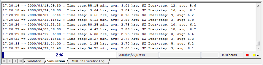
Run the simulation

In the Toolbar, click on the Water Movement icon to run the simulation.

This will start the MIKE Zero Launch utility.

Click OK

The Launch utility allows you to change the CPU Priority and the Results Folder prior to the start of your simulation.

You can also change the CPU Priority during the simulation by clicking on the yellow button in the lower right corner of the user interface. You can stop the simulation entirely by clicking on the red button.

View the results

Upon successful execution of the model you are now ready to view the results. First you should check the model run log files (.log) to ensure the model finished without any errors. The result files and log files are by default located in the Result folder under MIKE SHE exercises.

Go to the results in Result\YourFilename.she - Result Files folder (e.g. Result\Karup_basic1.she - Result Files folder) and double click on YourFilename_WM_Print.log

Scroll to the bottom of the file and check whether the different model components converged. Note that maximum iterations for some of the components may have been exceeded. This could be an indication of mass balance errors and we will check this when we create the water balance.

Locate the Detailed Time Series output results

After successfully running the model:

Click on the Results Tab located at the bottom of the Navigation Tree and select Detailed WM Time Series.

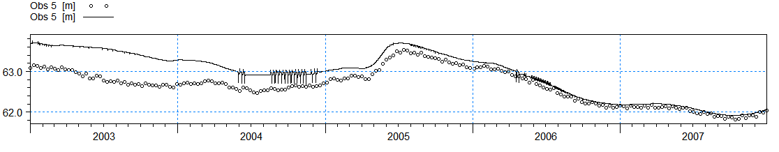
All of the observations should also be visible.

You can add additional detailed time series items now and re-run the model.

The Detailed Time Series output Dialog, under Simulation Results, lists the Detailed Time Series results you have chosen to store during the MIKE SHE simulation.

If you have specified more than 5 items for detailed time series output, then you will only see a page of links on the main Detailed time series page. The links will direct you to separate .html files with 5 graphs in each.

To plot multiple items on a graph, you can use the New Plot column in the Setup to combine output in one graph. If you unclick the checkbox, then this item will be plotted on the same graph as the previous item.

Locate the MIKE+ Detailed Rivers Time Series output results

Similar to the groundwater levels, find the MIKE+ (former MIKE HYDRO or MIKE 11) Detailed River Time Series.

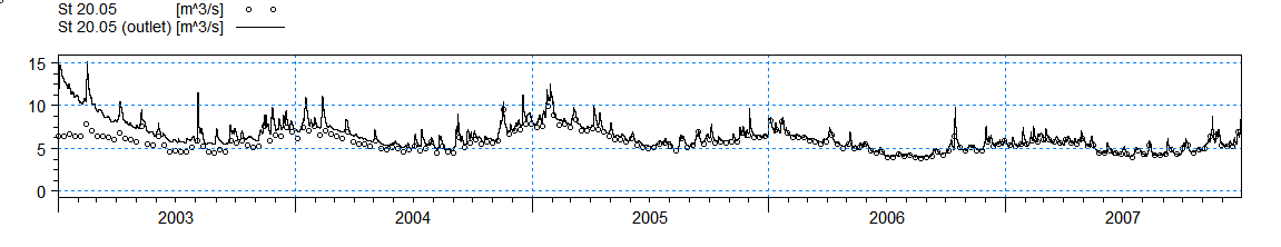
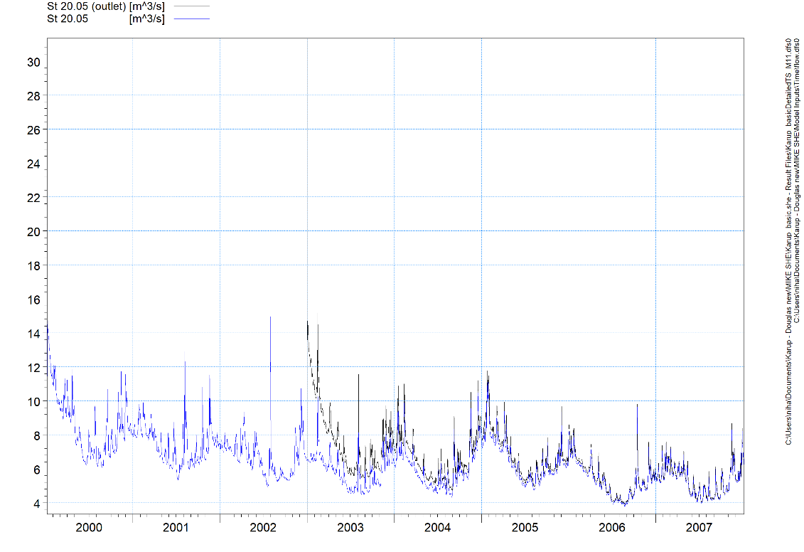
Plot flows using the Plot Composer

It can sometimes be difficult to see how well the model fits the observations on this graph. Alternatively try to use the Plot Composer for viewing the modelled and observed flow hydrographs.

To open the Plot Composer click New File on the main menu at the top below File

Select the Plot Composer

Click Plot->Insert New Plot Object and select Time Series Plot

Click New Item and browse to the result folder YourFilename.she - Result Files (e.g. Result\Karup_basic1.she - Result Files folder). Select YourFilenameDetailedTS_M11.dfs0 (e.g. Karup_basic1DetailedTS_M11.dfs0). Click the checkbox to select the item and click OK.

Click New Item again and add the observed flow data Model Inputs\\Time\\flow.dfs0

If you want, you can change the item names.

Click OK

To change the appearance of the graphs, right click on the graphs and select Properties (make sure you have selected the figure by clicking on it). Click Curves and change line colours and markers.

In the X-Axis and Y-Axis tabs you can change the length of the axes as well as some other settings.

To save the graph as an image click View->Export Graphics->Save to Bitmap

Save the plot composer file in the Model folder as Flow.plc

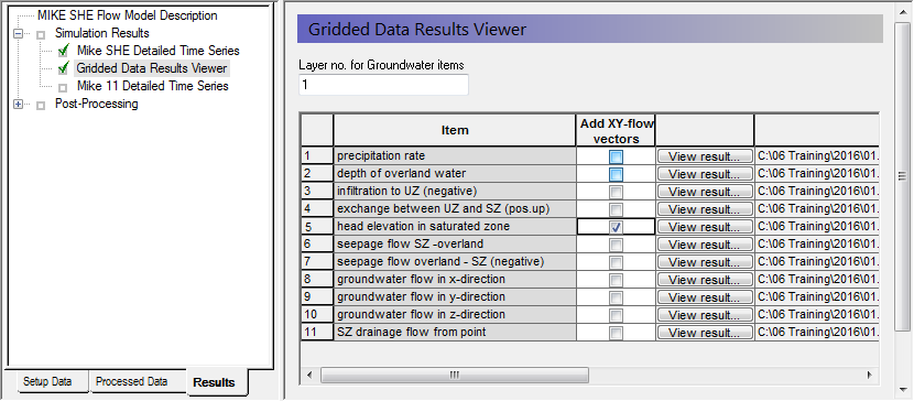
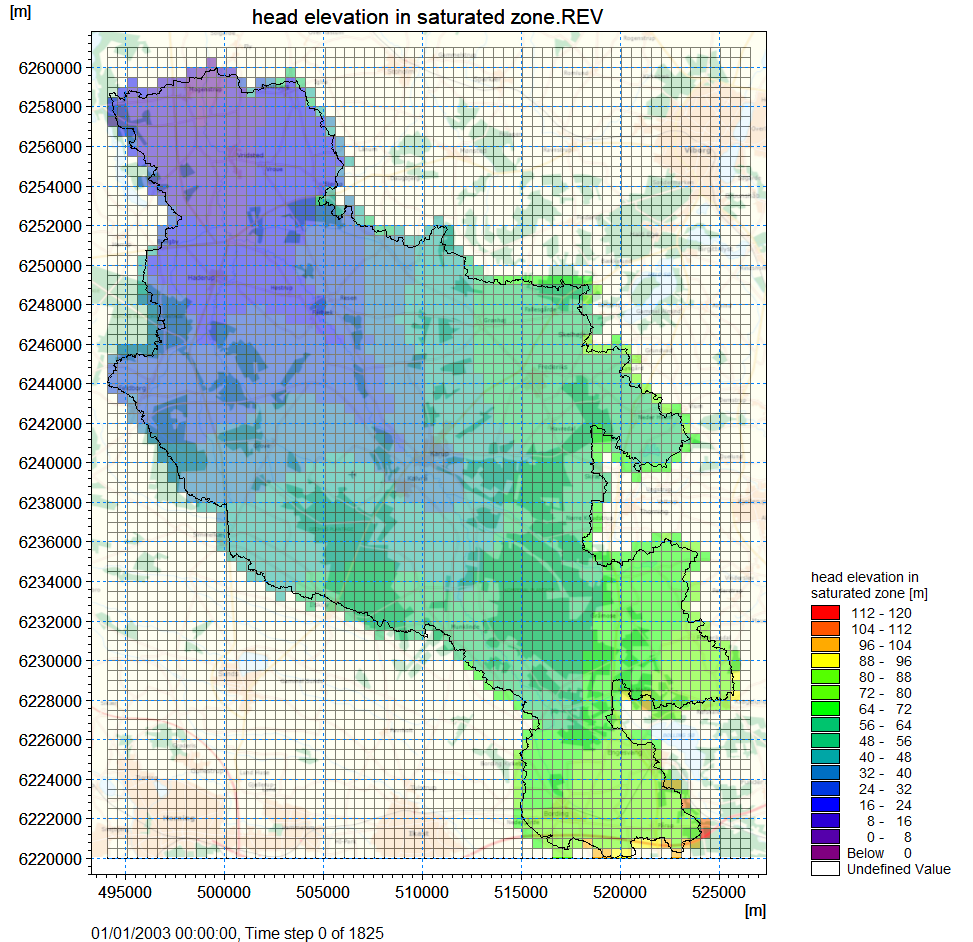
Display the gridded results

The Gridded Data Results Viewer dialog lists the results you have chosen to store in the MIKE SHE results files. The XY flow vectors check box adds groundwater velocity flow vectors calculated for each cell.

The Layer no for groundwater items in the top of the dialogue is used to select the numerical SZ layer number in groundwater outputs.

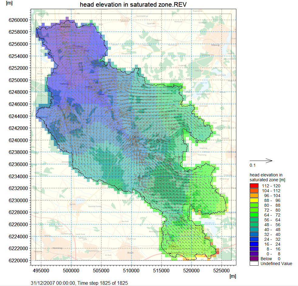
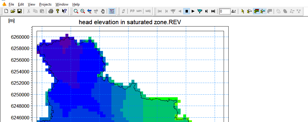
In the head elevation in the saturated zone item, check on the Add XY flow vectors for the plot and then click on the View result… button

Note

Note that the velocity vectors will not be visible in the initial time step, but appear in the second time step.

On the menu at the top:

you can play through the entire simulation, change the time step or create a video. To step through the simulation click on on the menu.

Note

Creating an .avi video is very time consuming, so don’t start the video creation process during a course.

Display a time series plot at a point

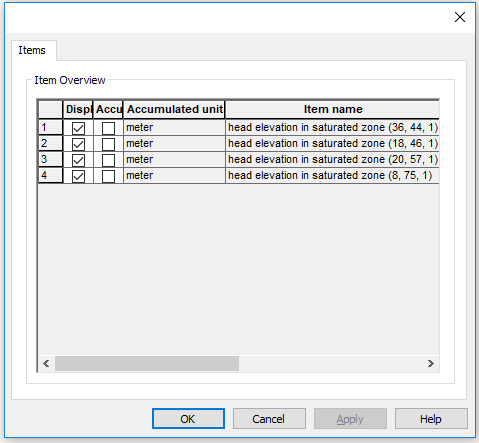
To view time series in points go back to the Gridded Data Results Viewer

Click View Result… for head elevation in saturated zone. Untick Add XY-flow vectors if these are ticked

Click OK when you are asked if you want to overwrite the existing file.

Click on the Time Series button on the Results Viewer tool bar

Click once inside the map area and then while holding down the Ctrl-key, click on each additional point where you want time series output. Each selected locations is marked with a yellow x.

Double click on the last point. (if you only want one point then simple double click without holding down the Ctrl-key)

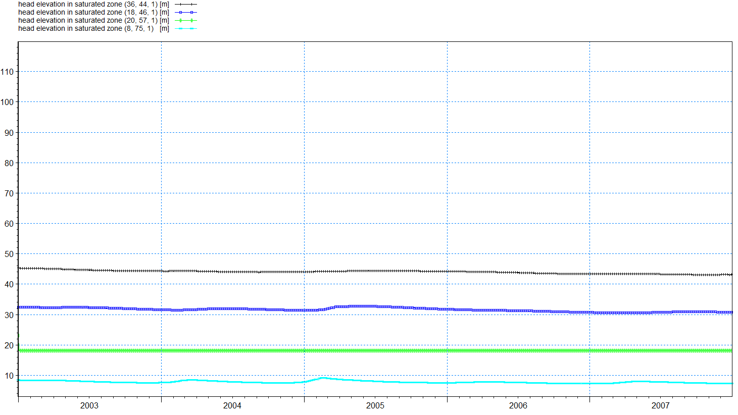
Check Display and press OK to display the time series.

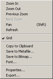
Export to a dfs0 file

• Right-click in the time series plot.
• Select Export… in the pop-up window.
• Check Export and press OK.

Enter an appropriate file name for the dfs0 file and press Save.

The (j,k) coordinates listed at the bottom of the Results Viewer go from 0 to (nx-1) and 0 to (ny-1) in the j and k directions, respectively.

Note

Note that the time series time steps are equal to the storing time steps. The Detailed timeseries output option within the Setup Data saves the output at every time step.

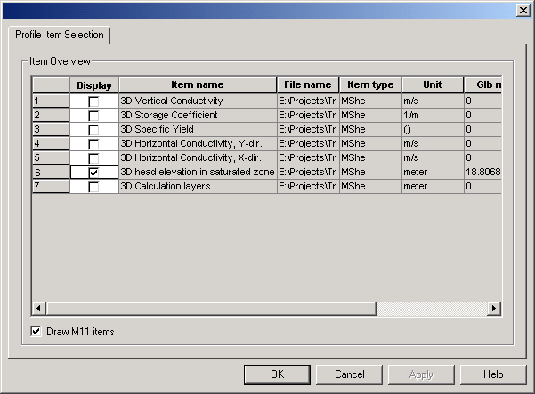
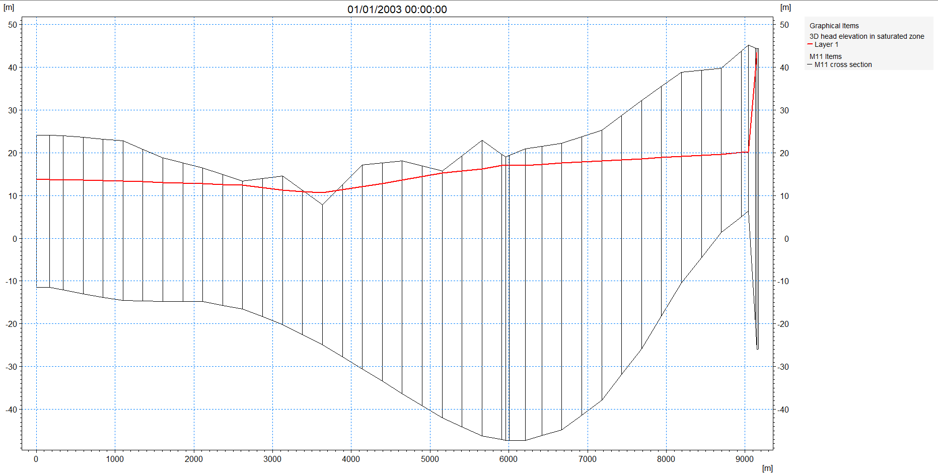
Extract a profile of water levels

Press the button on the Results Viewer tool bar to extract a profile from the simulate output item displayed

Click in the area of interest to select the points along the profile line. Double click on the last point of the profile to terminate the profile line. The profile line is indicated with a thick green line.

Check 3D head elevation in saturated zone and press OK.

To display the computational grid on the profile, in the Projects pull-down menu choose

Active View Settings -> Profile…

On the Graphical Items tab of the Dialog that appears, under Calculation layers,

Check Draw Calculation layer and select Draw as grid to show the computational grid or Draw as lines to show the upper and lower surface.

Press OK to view the selection.

Modify visible overlays and display the finite difference mesh in result viewer

First, return to the horizontal view of head elevation in saturated zone, by either closing the cross-section view or switching via the Window pull-down menu

In the Projects pull-down menu choose Active View Settings ->Horizontal …

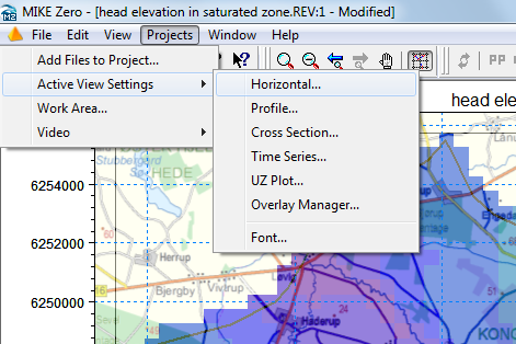
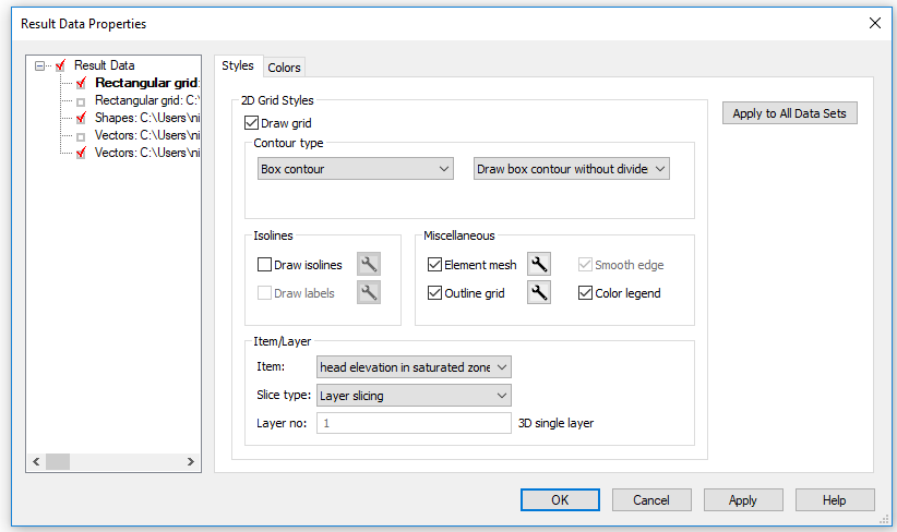
In the Dialog that appears

Single click on the Rectangular Grid item: YourFilename_3DSZ.dfs3 (e.g. Karup_basic1_3DSZ.dfs3) to view the available display options

Under the Miscellaneous items, check Element Mesh

Press OK to execute changes

Display other gridded data results

The number of gridded data items that are available depends on which modules were run and what selections you have made in the Setup. Many of these items are very useful for evaluating the integrated groundwater surface water interaction. You should explore some of these output items. For example:

Actual evapotranspiration – this is the sum of all the ET components. It is useful for evaluating the spatial distribution of actual ET.

Depth of overland water –typically this is a useful output for finding areas with permanently ponded water, or areas with closed depressions.

Seepage flow SZ – overland – this can be used for determining where springs are occurring in the model.

SZ exchange flow with river – this is useful to find losing and gaining river reaches.

SZ drainage flow from point – this output maps the locations where groundwater is contributing water to the SZ drainage network.

Total Recharge to SZ – this is a summary output map of all the items that contribute inflow to the SZ.

View simulation statistics

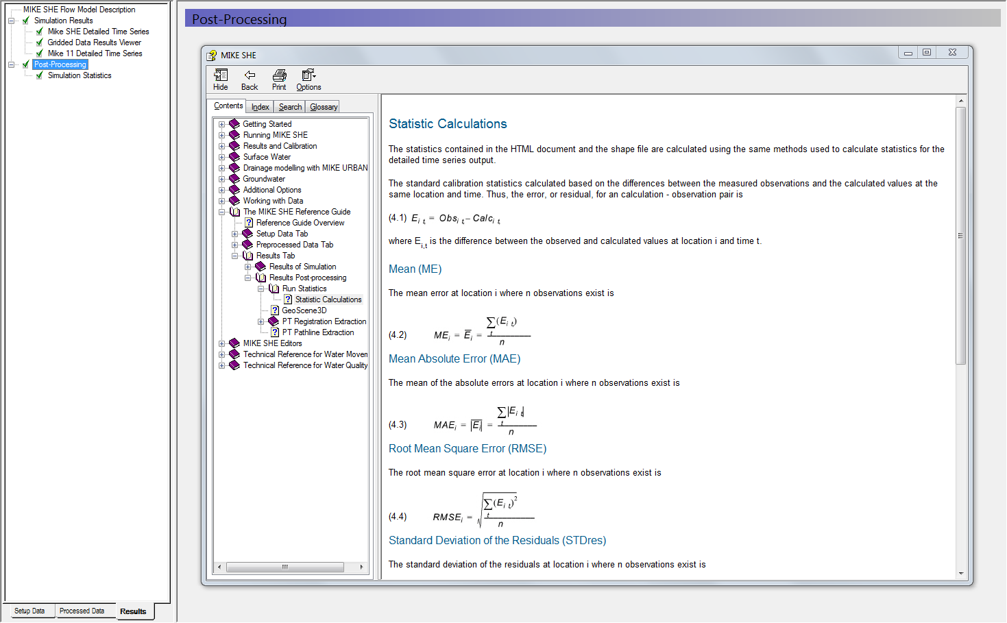
Statistics used for assessing the model fit are available in the Results menu under Post-Processing. The statistics are generated in HTML file format and include all the detailed time series items that have observation data.

The calibration statistics available comprise six standard statistics:

Mean (ME), Mean Absolute Error (MAE), Root Mean Square Error (RMSE), Standard Deviation of the Residuals (STDRes), Correlation Coefficient (R) and Nash Sutcliffe Correlation Coefficient (R2).

The equations for calculating the statistics are included in the Help menu and can be accessed by pressing the F1 key while placing the cursor over the Post-Processing menu

Note

Note that the statistics are calculated based on the differences between the measured observations and the simulated values at the time of the observations.

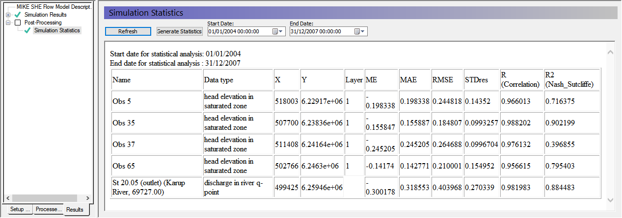
To generate statistics for the Karup model click Post-Processing->Simulation Statistics on the Results tab

Change the start date to 1/1/2004 and click the generate statistics button

Take a look at the statistics and assess the model performance

Check the water balance

The water balance utility in MIKE SHE is a vital part of the results analysis. The tool is versatile and can be used both for providing an overview of component inflows, inflows and storage changes over different periods and subcatchments and for troubleshooting any numerical issues.

Create a new water balance document

Click on the New document icon, , or the File/New/File menu

Select MIKE SHE and then the Water Balance Calculation (.wbl) document

Click OK

In MIKE SHE, water balances are calculated by the water balance utility. This is run separately after the simulation. Creating a water balance involves 3 steps:

1. Extract the water balance data from the MIKE SHE output files
2. Create specific water balances from the extracted data

Evaluate the water balance output

Extract the water balance data

Use the browse button and find the .sheres file from your simulation in your Result directory …\\YourFilename.she - Result Files (e.g. \Karup_basic1.she - Result Files)

Run the water balance extraction by clicking on the Extraction icon, or by selecting the drop down window Run and clicking on Extraction. You will be asked to save your water balance file. If the extraction icon does not appear at all, most likely the Run toolbar is not activated. Select the drop down window View, Toolbars and select the Run toolbar (last entry).

Check to make sure that the Extraction ran successfully, by looking for “Normal termination” in the message window

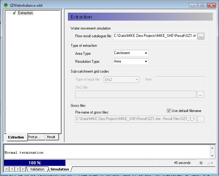
MIKE SHE saves the results in many different files. The results are grouped by process (e.g. OL, UZ, SZ) and by output type (i.e. 2D or 3D). The extraction process reads all of the various output files and builds a set of water balance files. These files can be efficiently read by the water balance utility.

The .sheres file is an ASCII catalogue of all the output files associated with the simulation.

The type of extraction is important, as it defines what subsequent water balances can be calculated.

Area Type – Choosing subcatchment allows you to create water balances for sub-areas in the model domain. Otherwise, the water balance is for the entire model area.

Resolution type – By default the water balance is for the entire catchment or sub-catchment. The Single-cell option allows you to create maps of some of the water balance items.

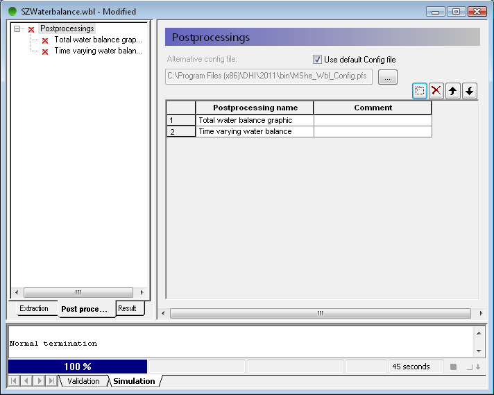
Create water balance items

On the Postprocessing tab, add two post processing items to the table by clicking on the new item icon,

Change the name of the two items, so that you can distinguish them from one another

You can set up any number of water balance calculations for a single water balance extraction. Since these are all stored in the water balance document (.wbl file), you can re-run the water balance extraction and processing after each simulation.

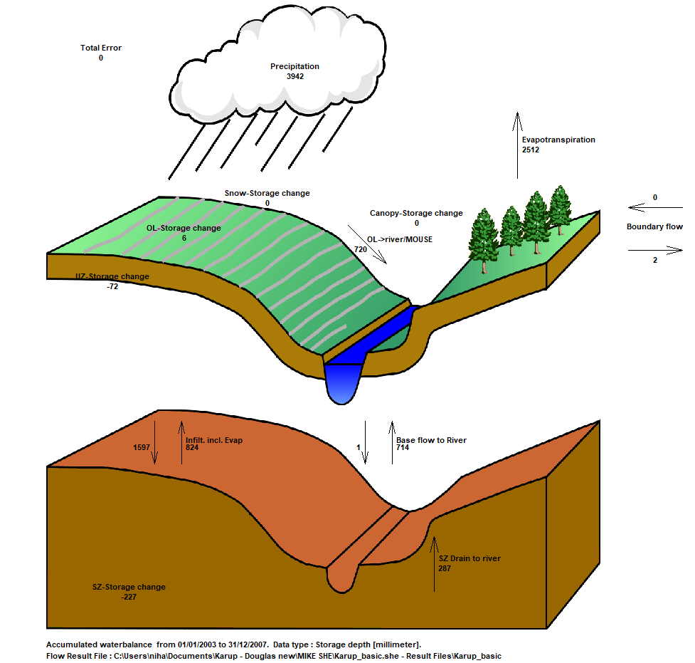
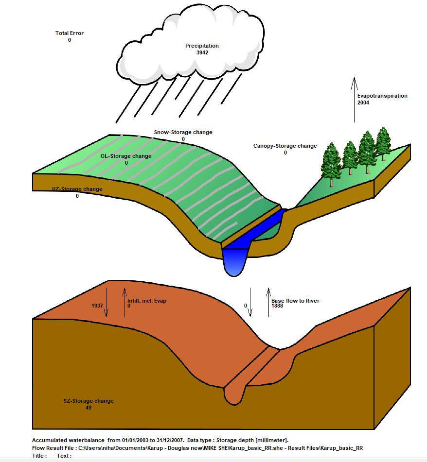
Define a Chart water balance

Select Chart output: Total water balance from the list of available Water balance types

Define a file name for the output file, for example TotalWB.txt. If you just type the name the program will automatically put it in the result folder

Run the water balance by clicking on the water balance icon run selected postprocessing,

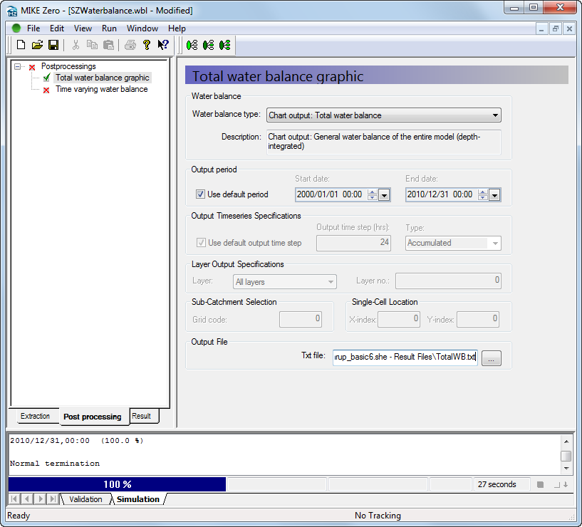
The Chart output creates a graphic illustrating the water balance items (see next step). The output is sent to an ASCII .txt file, and the graphic is generated automatically by a utility that reads the txt file.

By default, the water balance is summed for the entire simulation period. However, you can easily change the water balance period, for example, to create seasonal water balances, or to remove the initialisation period.

If you defined the extraction on a sub-catchment basis, then you can select from the available sub-catchments in this Dialog.

View the water balance output

On the Result tab, select the sub-item for the Chart output

Click on the Open button beside the file path to create and open the water balance graphic

To save the chart as an image file click File->Save Graphics… and select either Enhanced Metafiles (.emf) or Bitmap Files (.bmp)

The water balance graphic shown for the full model simulation period includes all of the non-zero water balance items in the current simulation (except for storage changes, which are always plotted).

The water balance items are all normalised to units of mm, which allows for easy comparison between the different components. If you want to convert depths of mm to volumes, you need to multiply the depth by the internal model area. That is, the total model area minus the area of the outer boundary cells. If you load the pre-processed data into the Grid Editor, select the Model and Domain item. Then, you can use the statistics function in the Grid Editor to find out the number of internal versus external cells.

Note

The sum of the water balance terms in the graphic do not add to zero. This is because some of the signs have been removed (e.g. Precipitation and ET have the same sign, but opposite inflow/outflow directions). In the water balance calculation, inflows are negative and outflows and storage increases are positive.

Define a time varying water balance

Return to the Post-processing tab and select the second water balance item

Select Total water balance from the list of available water balance types

Leave the Output type as Accumulated

Select the Output file type as a Time series file

Input a filename with the .dfs0 extension, for example TotalWB.dfs0. Unless you browse to another location, the file is automatically saved in the results folder.

Run the water balance by clicking on the run water balance icon

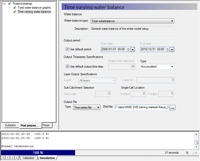
If you chose the Table format for the Output file instead, then the output will be in a tab-delimited ASCII file that you can open in Excel.

In this exercise we have chosen an Accumulated water balance. This sums the water balance over the simulation period.

The alternative is to define an incremental water balance, which outputs the water balance time series at each saved time step.

View the water balance output

On the Result tab, select the sub-item for the time series output, Time varying water balance

Click on the Open button beside the file path to create and open the water balance time series file (.dfs0)

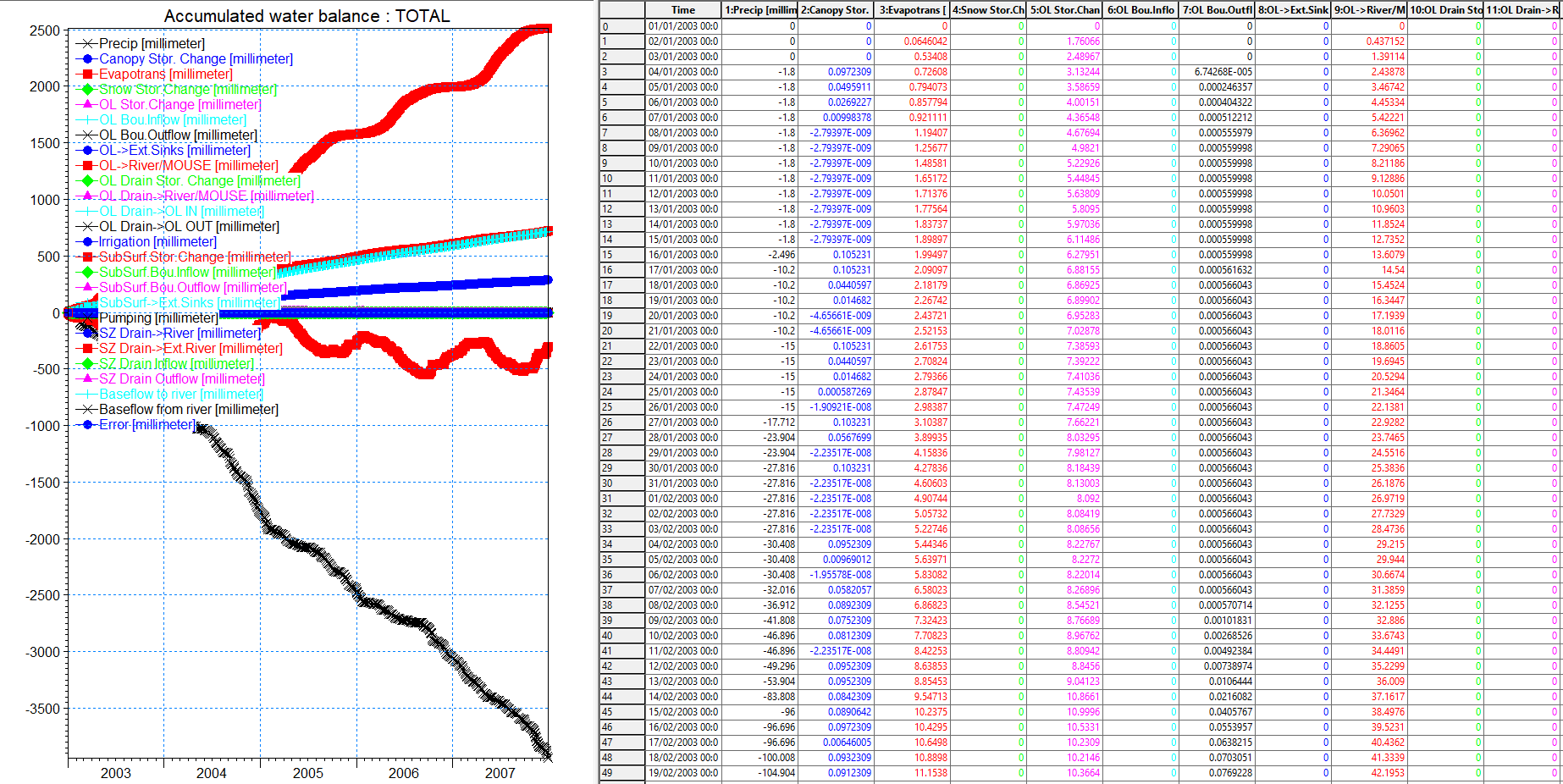
The water balance time series file includes all of the available water balance items – most of which are also shown on the chart of the total water balance.

The cumulative water balance sums the items over all of the stored time steps. Scrolling to the bottom of the file the total precipitation is the same as in the graphical total water balance chart above. Some items have been lumped together in the chart.

Note, that the sign of the precipitation is negative and ET is positive in the time series file. This is consistent with the water balance sign convention which is:

Outflow – Inflow + StorageChange = 0

Thus,

• All inflows to the model are negative
• All outflows from the model are positive
• A negative change in storage means that water is accumulating (an ‘Inflow’)

A positive change in storage means that water is draining (an ‘Outflow’).

One important thing to remember is that the water balance is only an output of the saved time steps. Thus, the dynamics between the saved time steps are lost.

Building a MIKE+ Rivers Model for MIKE SHE

The purpose of this exercise is to get to know MIKE+ Rivers by inspecting and completing a MIKE+ Rivers model for a MIKE SHE model. The model is based on the stream model for Karup used in the Karup integrated MIKE SHE exercise. The exercise covers the following topics:

• Adding a river branch and boundary conditions
• Generating cross-sections from a DEM
• Routing vs dynamic branches
• Adding a weir
• Model stability
• Using MIKE View for result processing
• Demo Note: The MIKE+ Rivers setup has too many elements for you to save the model. You can follow the steps in this section for practice, but you will not be able to save or run the model with the changes.

Open the MIKE+ Rivers model setup file

Ensure that you have installed the MIKE SHE Examples files in the previous Getting Started exercise. Open the MIKE+ Rivers model by double clicking on the Karup_basic.mupp file. This could take a few seconds.

The MIKE+ interface is a bit different compared to the MIKE SHE (or MIKE HYDRO or MIKE 11) interface, but is more map-oriented. It includes all the model settings and parameters on the left pane (although all windows/editors are fully movable and can be docked anywhere in the GUI).

A map of the river setup is shown in the middle window. It is possible to shift between the map and tabulated values by clicking on the ‘Map’ tab (or by selecting ‘Map view’ at the ‘Project’ menu) or at any Setup item to display the respective editor in the middle view (new tabs are created with associated editor windows). You may also want to drag and dock a certain parameter editor window and place it next to or above/below the Map view.

Model components/parameters can be selected either on the left pane or by switching between the different tabs at the middle editor view. Details and available properties of the different model components may be shown in the pane to the right of the map/editor window by selecting ‘Property view’ at the ‘Project’ menu.

Icons for zooming in/out and for inspection of stream parameter values are available from the ‘Map’ menu (Navigate ribbon) or at the toolbar on the top of the Map view.

Validation of the data inputs is carried out when opening the model but can also be issued from Simulation specifications > Simulation setup > General tab > click on the ‘Validate’ button. The ‘Log View’ at the bottom (if not displayed can be called from ‘Project’ menu) shows model related information such as relevant warnings when failing to load map layers while opening the model setup at the beginning.

Click on Map view and select ‘Zoom full extent’ for a visual inspection of the river setup.

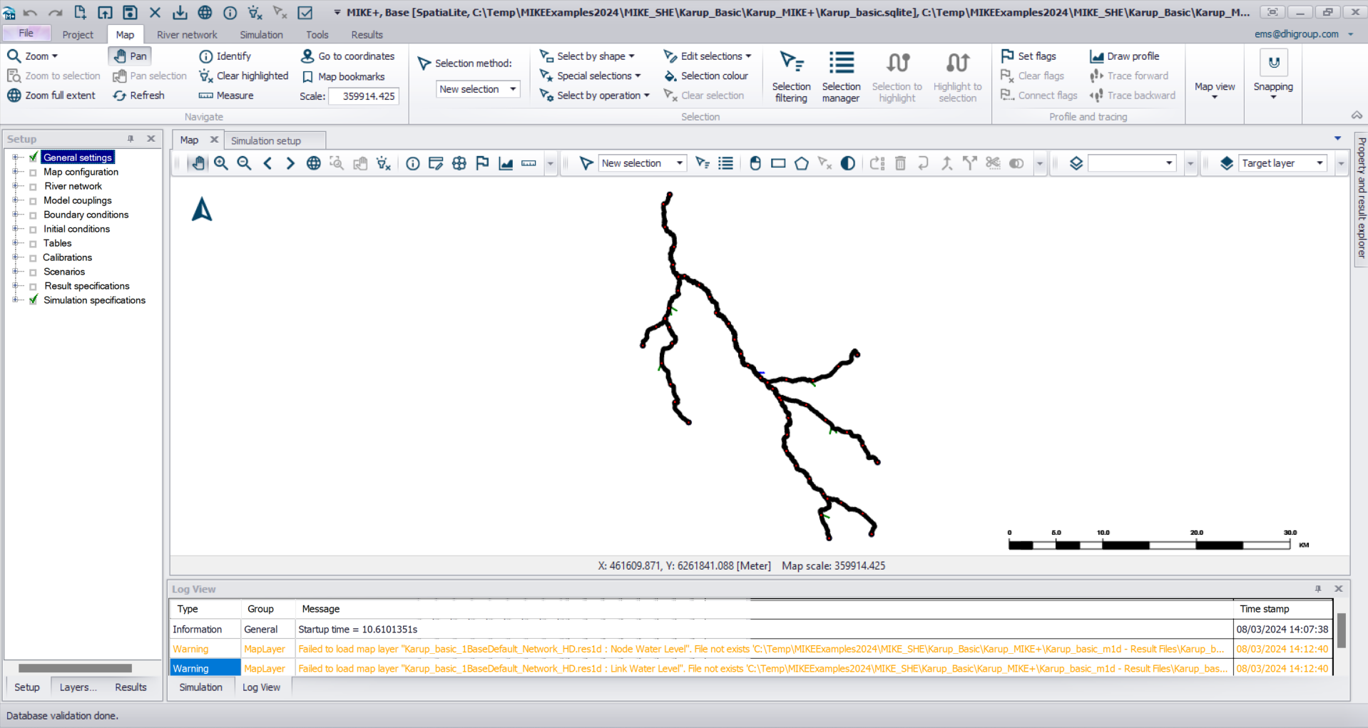
On the left/Setup pane the ‘Model type’ under ‘General settings’ allows you to select the type of Features and Modules to include in the model setup. In this case the River network and the Hydrodynamic (HD) Module have been selected. Depending on the selections, different data input editors will be available at the Setup pane.

• The simulation period and time control are specified at the ‘Simulation setup’ editor under ‘Simulation specifications’. However for a MIKE SHE model run the simulation period is overridden by the simulation period specified in the MIKE SHE menu (see 3.3.2).
• ‘Map configuration’ allows you to specify the coordinate system and include background maps.
• ‘River network’ includes details of the river network including any structures. It also contains the ‘Bed roughness’ parameters.
• ‘Boundary conditions’ include the river network boundary conditions.
• ‘Groundwater couplings’ under ‘Model couplings’ allows you to specify the couplings with MIKE SHE.
• ‘Initial conditions’ allows for initial flows and water levels to be specified.
• The ‘Simulation setup’ Results tab allows you to set the output file name and storing frequency for the output, while the results items and any additional result files can be specified at the ‘Result files’ under ‘Result specifications’. In dynamic simulations the time step for MIKE+ Rivers can be quite small, so it is often necessary to reduce the storing frequency.

Set the results directory

The current results directory can be changed under ‘Simulation specifications’ ->‘Simulation setup’ ->‘Results’ tab

Ensure that Save results in default folder is selected

This will create a result folder using the MIKE+ Rivers name: Karup_basic_m1d - Result Files located under MIKE SHE exercises. You can select a user defined folder instead but make sure you use a sensible name.

Leave the ID unchanged - it will be used for the results file name

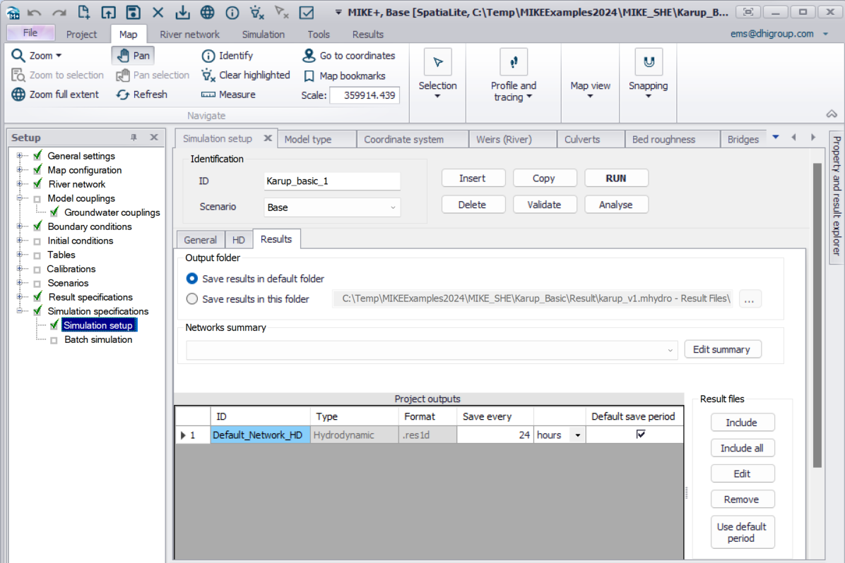
Explore the branch network and add a branch

On the Setup pane click on River network ->Rivers. Also select the River network menu at the top to show the rivers-related ribbons and tools.

Inspect the stream network in the map view.

The appearance of the river can be modified by switching from the Setup pane to the Layers and symbols tab/pane on the bottom left. Select River > Rivers > Default to change symbols and labels for rivers, river connections or user defined chainage points.

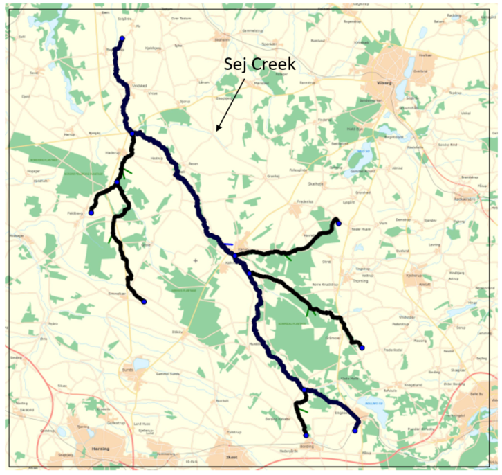
One tributary named Sej Creek is currently missing in the river setup. The river branches are shown on the background map as blue lines.

• Add the missing branch by clicking Tools menu ->Import and export ->
• Add job
• Source type: Shape file: browse for .\Karup_Basic\Karup_MIKE+\GIS data\Sej.shp ->Target type: MIKE+ DB
• Insert section
• Source: Sej ->Target: mrm_Branch ->Transfer mode: Append & Skip existing
• Automap
• End chainage: BRS_end ->Start chainage: BRS_start ->geometry: geometry ->MUID: RiverName ->TopographyID: Topo_ID
• Verify ->Run ->Close

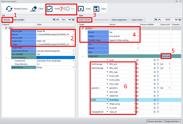
Convert the branch from Dynamic to Routing

Select Rivers under River network to open the Rivers editor and view the branch details.

Change Sej creek from a Regular branch to a Simple routing branch in the River type field in the Rivers editor > Geometry tab (do not worry about the red exclamation mark in Topo ID for the moment)

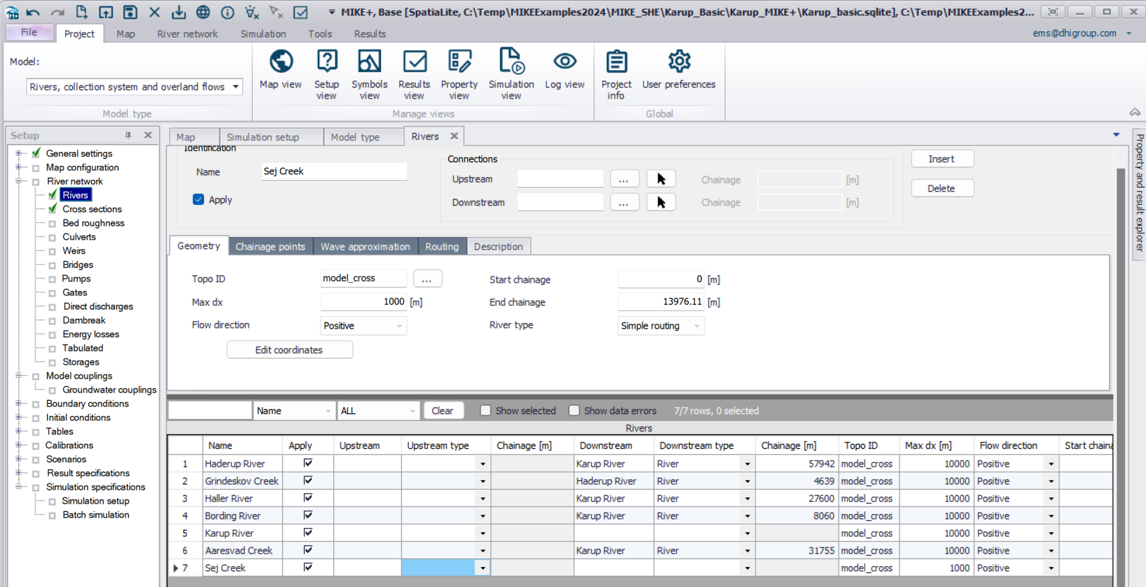
A regular branch will calculate the water level based on the Saint-Venant equation (Kinematic, Diffusion or Dynamic Wave formulations). For detailed simulations, you would generally use regular branches.

However, often it is convenient to use simpler routing formulations, where the water in the river is moved down the river – without actually calculating the water levels. Water levels are calculated afterwards knowing the flow rate in the cross-section and back-calculating a water level.

The main advantage of the routing methods is their speed. They require less data, they are numerically stable and you can use long time steps if you want.

The downside is that the calculated water levels are less precise and hydrodynamic effects are ignored. Water levels are simply calculated based on the amount of water in the river in the current time step.

You may also combine different approaches, for instance by using simple routing techniques on the upstream, steep branches and the dynamic wave method on the downstream low-gradient branches.

For simplicity and to ensure the model runs fast, the existing branches (at least the tributaries) have all been set as routing branches.

Connect the branch to the Karup River

Return to the map view and

Zoom to the confluence with the dragging zoom function in the icon bar

Connect the branch to Karup River by clicking at the River network menu > set the Target layer to: River connection > click on the Create button , then clicking on the end of the Sej Creek branch and dragging the cursor anywhere on the Karup River (you will see a small white circle appear on the Sej Creek, then connect to any point along the Karup River, while doing so you may notice that snapping becomes active).

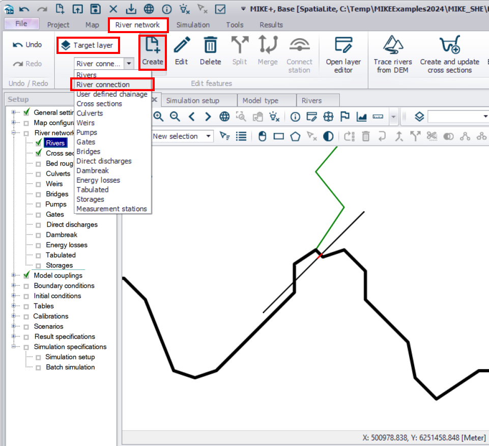
Now, go to Rivers editor and change the downstream connection chainage for Sej Creek to chainage 57054 (the location of an existing cross section)

Routing methods

To view the routing method parameters go to Rivers network ->Routing method Dialog.

On the last entry select Sej creek and the Routing tab to switch to the Routing parameters editor. No changes will be applied in this case (which means that the outflow from the specific river branch will equal the inflow).

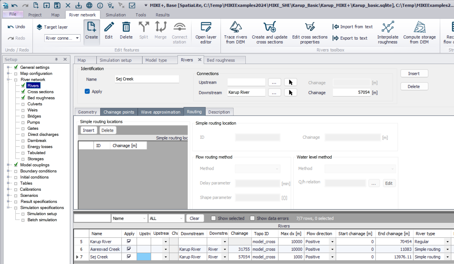
In the Routing Method Dialog normally you only need to specify a chainage close to the end of the branch. If no other specifications are made, the model will:

Calculate water levels using the Manning Equation assuming that the energy slope equals the bed slope derived from cross-sections (Manning numbers are specified in the Bed roughness parameters editor, default is M=30 [m1/3/s], n=1/M).

Use the ‘No flow routing’ method, which implies that inflows are summed along the branch and transferred to the downstream end of the branch in the same time-step. This is the same as a full pipe with a unit of water entering one end and pushing a unit out the far end.

Another discharge computation option is the Muskingum methods. It dampens the peak flows as they travel downstream, which is necessary when the travel time in the river is much longer than the time step. For example, in large river networks, it may take several days or longer for a flood wave to travel from the source to the river mouth.

augNote: In the Simple routing option calculations are only performed at cross section locations. The Maximum dx = 1000 m specified in the Rivers editor parameters on the Geometry tab is not used. You may include additional routing points at different locations along a branch, but this will not be covered in this exercise.

In this exercise, you are using the simplest option, where no routing is used. Thus, whatever water flows into the branch network at the boundaries or as lateral inflow, will be transferred downstream in the same time-step.

augNote: MIKE SHE keeps track of and conserves mass and does not allow water to infiltrate from the river to the groundwater if the river is empty.

View and add cross-sections from a DEM

Cross section data can be accessed by selecting Cross sections under River network at the Setup pane on the left or by selecting the Cross-sections tab at the top of the middle view in case the Cross sections editor has already been opened. Active cross sections extents (within markers 1 and 3) are displayed with red lines on the map, while full cross sections widths (from Raw data tab) are displayed with black lines.

Note

The cross section may be difficult to see with the default symbol (black line). It may therefore be necessary to change the Symbology to show the cross sections with dots first.

Cross sections are saved to a cross-section file .xns11 (see the General tab) which can only be viewed and edited using the MIKE+ GUI Cross sections editor. To view the file in the Cross sections editor you first need to open MIKE+ software and create a new or open an existing MIKE+ project.

In the Cross sections editor,

• Cross sections are identified by a River ID and a TOPO ID
• Cross sections data are relative to the specified Datum value
• Cross sections data are editable in the table

The marker values 1 and 3 in the table define the extent of the cross section (left and right banks, respectively) to be used in the simulation

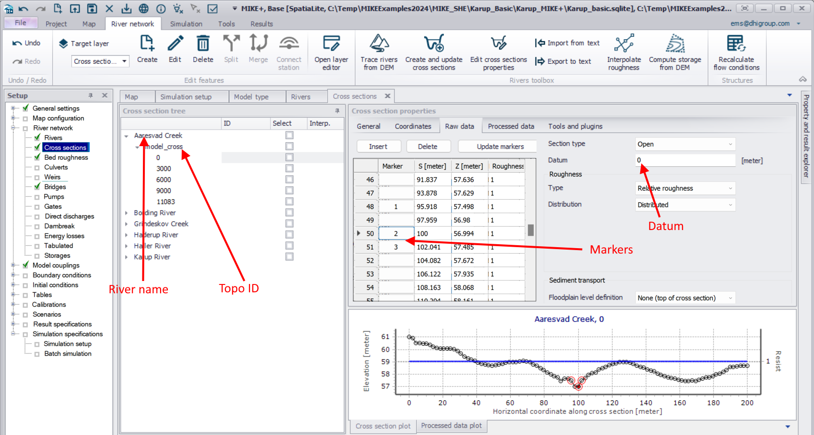
Cross sections for Sej Creek need to be added to the model setup. Survey data are not available but a detailed Digital Terrain Model (DTM) can be used instead. For this exercise the DTM was resampled (from 1.6 m) to 3.2 m to keep the file to a reasonable size. Note the example cross sections file included with the training material was generated using the original file with the fine resolution.

You may want to load a background map, such as Open street map or Google maps that can be displayed on the background. To do this you first need to set the Coordinate system under Map configuration at the Setup pane and browse for the projection: ETRS_1989_UTM_Zone_32N (Tip: at the Map Projection Editing dialog click the Find button and enter the projection name).Then, at the Background map under Map configuration you can select the Background map overlay e.g. Open street map (Tip: if the Open street map and Google maps options are still deactivated you may need to save, close and reopen the MIKE+ model setup).

Go to Layers and Symbols ->Add layer… ->Layer type: Raster layer ->Raster file type: Raster text files ->Browse and select .\GIS data\Sej_DEM.asc. ->set the Z-value unit to meter and click OK. This may take a a few seconds as the file is large.

Click Map to view the DEM.

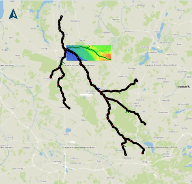
A DEM can be defined in various file formats including ESRI ASCII, dfs2 or GeoTiff files. For ESRI ASCII files the coordinate system and z unit for the file must be specified. If a .dfs2 is chosen these parameters are taken from the dfs2 file definitions.

Before saving the model create a backup of the original cross section file and save with a new name. In Windows explorer go to the folder location, right click on Karup_basic.xns11, copy it, and then change the name to Karup_basic2.xns11. browse for Karup_basic2.xns11.

Go back to MIKE+ and save the model as Karup_basic2.mupp

At the Cross sections editor select Karup_basic2.xns11

To extract cross sections for Sej Creek select River network menu ->choose Create and update cross sections at the Rivers toolbox ribbon

Choose Method: Create or extend cross sections from DEM

DEM settings: DEM layer: GIS data\Sej_DEM.asc

Keep the default values for Maximum spacing between points and tick Use bilinear interpolation from 4 closest cells

For Cross section location choose the option Create new with constant lengths and specify an interval of 3000 m and a width of 100 m

For Input selection and River selection choose the option Single river: Sej Creek

Click Run and Close the window

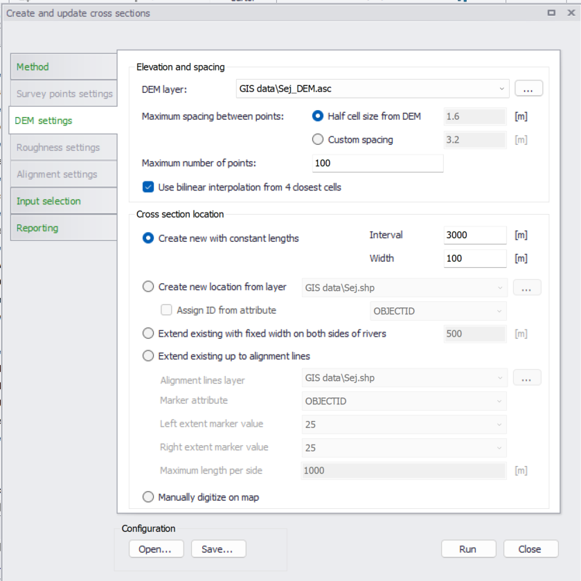
Click on the Map to view the location and length of the cross-sections.

At the Cross sections editor and the General tab ->Recompute all to compute processed data for all, including the new, cross sections

The cross sections are too wide and only the main channel geometry should be included in the model. To constrain the extent of the cross section used in the simulation the bank markers will have to be moved. This can be done in different ways. Embankment lines can be defined either as shapefiles or by digitising them in MIKE+. Alternatively the markers can be modified manually directly in MIKE+. For this exercise the cross sections will be modified manually in MIKE+ by modifying accordingly, markers 1 and 3:

Go to River network -> Cross sections editor

Click Sej Creek (Topo ID: model cross) and select Chainage 0

On the Cross section properties menu select Raw data

Sej Creek is quite small and the DEM is not sufficiently detailed to include the channel everywhere. As a guide set the width to app. 5-20 m.

On the displayed cross-section, you may need to enlarge the view by dragging the window bigger. If more than one cross-section is visible, you can remove all but the current one by right clicking on the cross-section plot and selecting Clear history.

Click on a point in the cross-section that you want to define as the left hand top-of-bank. Then, under Marker in the table, click on the highlighted box, . (The point will be red in the cross-section plot).

In the dialog that appears, chose the (1) Left levee mark.

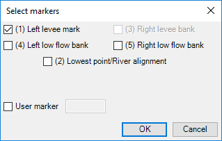
Do the same for the bottom of the stream (2 Lowest point/River alignment) and right bank (3 Right levee bank)

Repeat the process for all the cross-sections in Sej Creek

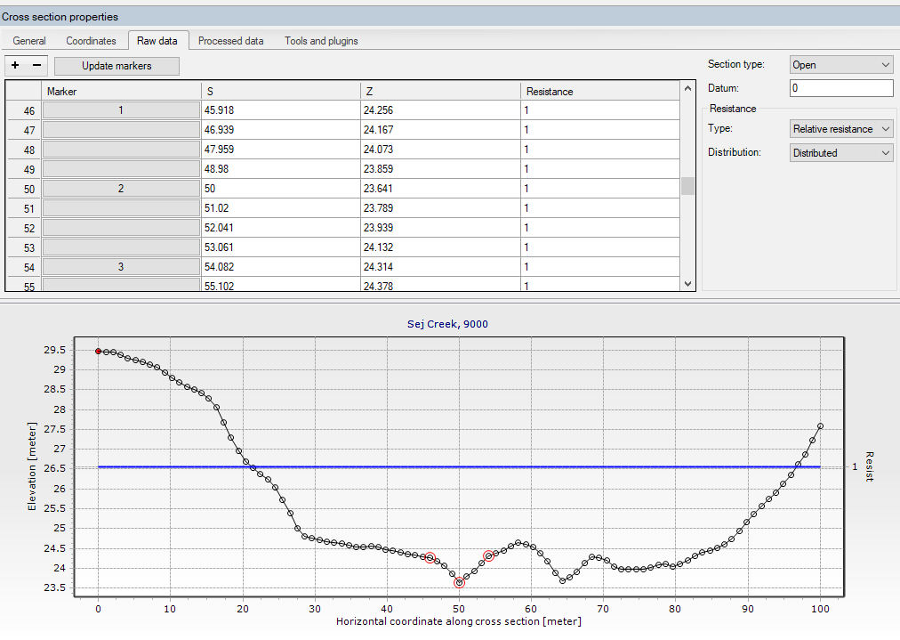
To ensure that the rivers fit together at the inflow of Sej Creek into Karup River, copy the cross section from Karup River at 57054 m and insert into the end of Sej Creek (you need to double check the end chainage for Sej Creek in Rivers editor, it is important that they are identical up to 2nd decimal digit) by right-clicking on the cross section at 57054 m, choosing Copy and then filling out the Copy dialogue:

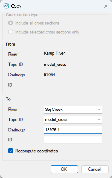
Save the MIKE+ project.

Add boundary conditions

Boundaries can be viewed by selecting Boundary conditions -> Boundary conditions at the Setup pane on the left. The boundaries are shown with dark red dots on the map.

Now take a quick look at the boundary specifications in the model. All the upstream ends (Chainage = 0) are defined as Inflow boundaries with very small inflow. The downstream mouth of the river is defined as a Q/h relation.

Add another Inflow boundary for Sej Creek (Chainage = 0) with zero inflow by selecting the Insert button at the Boundary conditions editor and change the Type from the default Inflow from result file to Open inflow to river

At the Spatial extent tab choose the option Individual, click on the browse button and choose the Sej Creek river. For Chainage keep the default option Start chainage

At the Temporal variation tab choose the Time series option and click the Browse button. Navigate to .\Karup_MIKE+\karup.dfs0 and choose the default item q=0. This specifies a very small inflow of 0.005 m3/s, which will reduce the risk of the model running dry

Specifying a small influx as a boundary condition will prevent the model from running dry and will also keep the model more stable. This is only an issue when using a regular branch with Kinematic, Diffusion or Dynamic Wave formulations.

Run a simulation

To test that the model has been set up correctly, it is necessary to run the model. This section shows you how to run MIKE+ without MIKE SHE. This is a good check to ensure that your MIKE+ Rivers model works correctly. If you want to run the models coupled, just start the MIKE SHE simulation as you did in the previous exercise.

In MIKE+, run the model by selecting Simulation setup (under Simulation specifications in Setup pane on the left). A simulation scenario (named Base with ID: Karup_basic_1) has already been defined. At the General tab make sure River network and Hydrodynamic (HD) options are checked under Simulation type Features and Modules, respectively

You may want to click the Validate button to check for any validation messages before clicking the RUN button to run the simulation

Inspect the run messages on the Simulation pane and make sure the model run finished without errors

If you want to get more interesting results, you can add more water through the inflow boundaries.

• Navigate to Standard Boundaries in the Setup-tree and choose tabular view
• For each inflow boundary condition, navigate to the file .\inflow.dfs0 (located together with the Karup.dfs0 file that you have previously used)
• For Karup River choose the item “Inflow main” and for the remaining branches choose “Inflow tributaries”
• Remember to change the boundary conditions back before running the model coupled with MIKE SHE!

While this adds more water to your model, there will still not be a lot of variation when MIKE SHE is not included, as you are adding a constant discharge and have no variations caused by precipitation, evaporation, infiltration etc. However, it will show you more clearly the effects of different changes made to the model, for instance adding a weir as described later on.

For a fully hydrodynamic solution it is sometimes necessary to run it with an inflow hydrograph upstream in order to test whether the model is stable for the full flow range. It is also recommended to generate a result file with small boundary inflows that can be used as a HOT-start file to prevent initial instabilities.

Remember to export the river model to .m1dx file (File menu -> Export). This is a prerequisite by MIKE SHE (at the Rivers and Lakes editor) in order to run a coupled simulation with MIKE+ Rivers.

View the results

To check the model results, open MIKE View by going to the Start menu and select MIKE View 2024 -> MIKE View

Load the results by selecting the file type as .res1d and the select your latest simulation results.

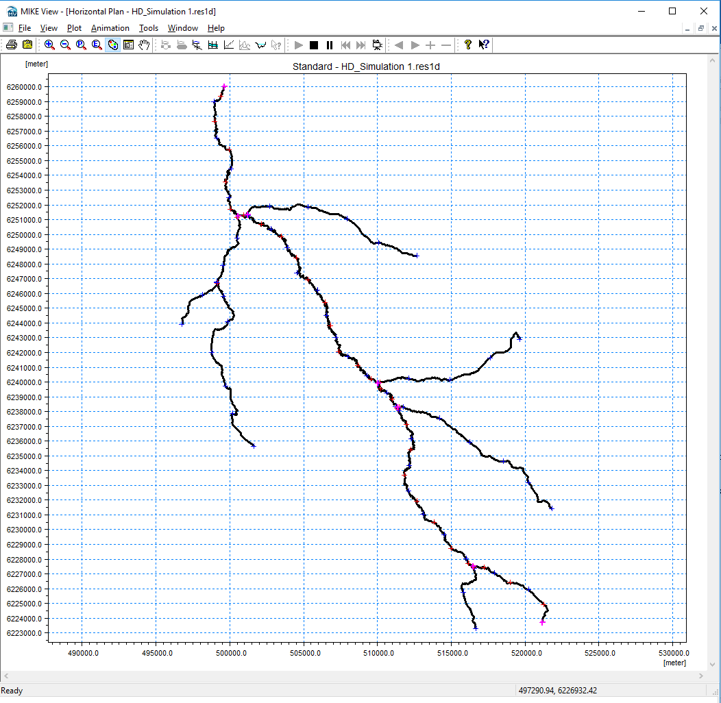
Click to select and plot a time series of discharge at the downstream confluence. This should show a constant stream flow of 0.035 m3/s

Click and select a branch to plot a cross section showing the water level. Click on the branches you want to view and press the Ctrl key and click in the view to complete the cross sectional plot

Click to run through the simulation and to pause at a desired time

The result below is from running MIKE+ Rivers coupled with MIKE SHE.

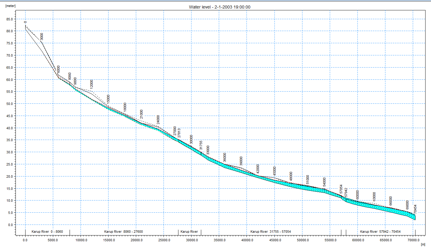
MIKE+ Rivers – MIKE SHE coupling

Before running MIKE+ with MIKE SHE, you must ensure that the new river tributary is coupled to MIKE SHE. In the Model couplings -> Groundwater Couplings editor, you specify which MIKE+ river branches will be coupled with MIKE SHE. You may choose to include some of the river branches or all of them, or even just part of a branch.

Add Sej Creek by clicking the Insert button and browsing for Sej Creek in the River ID field

Ensure DS chainage is set at at the end of Sej Creek river (in this case 13976.11 m - you may need to check the end chainage in the Rivers editor) to couple the full length of the branch to MIKE SHE

Keep the default conductance option (Aquifer + river bed) and leakage coefficient (10-5 sec-1)

The coupling specification includes the definition of the river-aquifer exchange, including the river bed leakage coefficient. The river leakage can also depend on the hydraulic conductivity of the aquifer material when the MIKE SHE cell size is much bigger than the river width.

The exchange between MIKE SHE and MIKE+ Rivers is one-way (default setting). Overland surface water from MIKE SHE will flow into the MIKE+ river, but water will not flow back onto the ground surface if the river floods. Overland flooding can be included, using one of two options:

Cells can be defined by flood codes, where they will be flooded if the elevation of the MIKE SHE cell is below the water level in the nearest river H-point.

Alternatively, you can allow overbank spilling. In this case, the river will discharge the water onto the ground surface based on a weir formula.

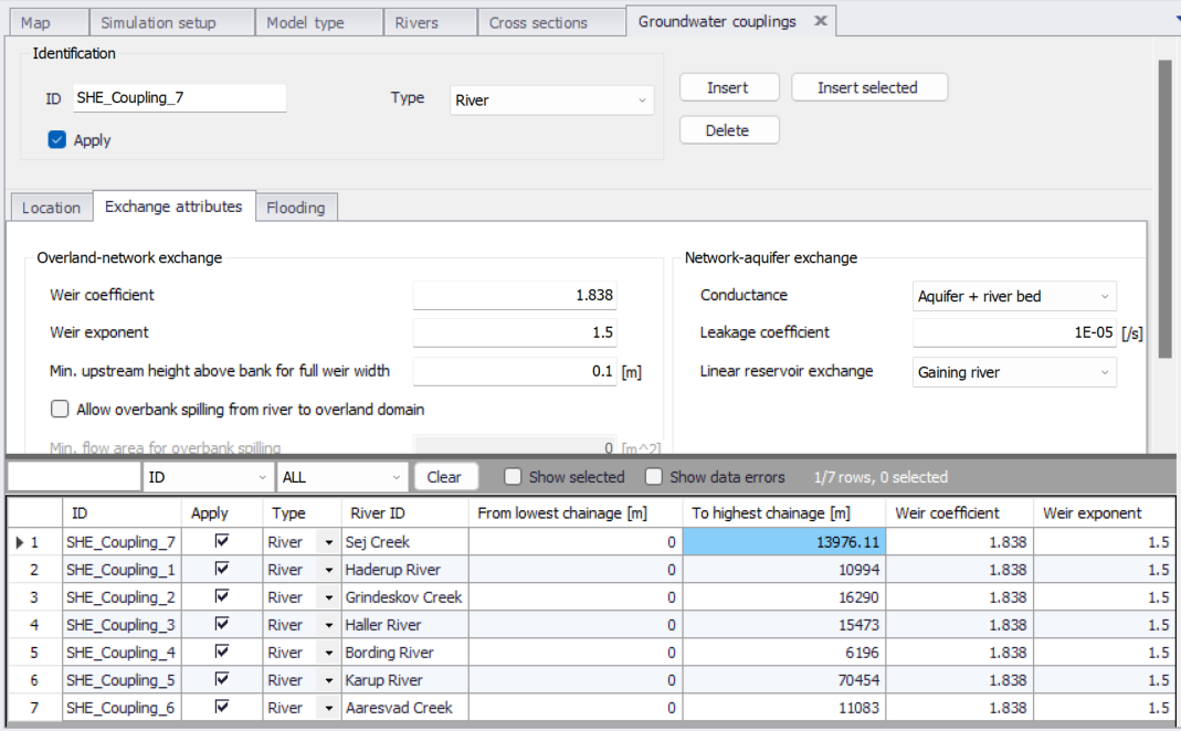
You will run the MIKE SHE model in the same way as you did in the previous exercise. First

open the Karup_basic.she model or your own model from the previous exercise. Remember to change the name to e.g. Karup_basic2.she.

change the river input to the MIKE+ exported river model Karup_basic2.m1dx you have created in this exercise.

Change the simulation period to 1 year (End Date: 31/12/2003) and run the model

Add a weir structure

You will now add a weir to the main branch Karup River. The weir is a broadcrested weir located at river chainage 29950. The width is 2 m and the sill level is 31.5 m AOD.

Add the weir dimensions

A number of different weir formulations are available: Broad Crested, Villemonte Formula, Honma Formula and Extended Honman Formula.

The geometry for broad crested weirs can be defined in two different ways:

Level-Width: The weir geometry is specified as levels (relative to the datum) and corresponding flow widths. The widths therefore define the area in which water can flow, and the datum is the bottom level of the opening.

From topography file: The weir geometry is specified as a cross section in the cross section editor. A cross section with a matching river name, Topo ID and chainage must exist in the applied cross section file.

Note: Since a weir is defined as a structure causing a contraction loss and subsequently an expansion loss, the geometry of the weir must be such that the cross sectional area at the weir is less than the cross sectional area at both the upstream and the downstream cross section for all water levels.

You can now add the weir. In this exercise, the weir geometry uses the Level-Width option:

First save the model with a new name, e.g. Karup_basic2weir.mupp

Go to River Network -> Weirs

On the Geometry tab click the Insert button to add the weir and change the ID to Karup_spill

At the River ID browse to the Karup River and set the chainage to 29950

Leave the Weir type unchanged (Broad Crested)

Under Geometry type select Level-Width (default) and set the Datum (sill level) to 31.5.

For the Level-Width relationship specify the weir dimensions by clicking the Insert button adding three lines:

• Level=0, Width = 0
• Level=0.1, Width = 2
• Level=10, Width = 2

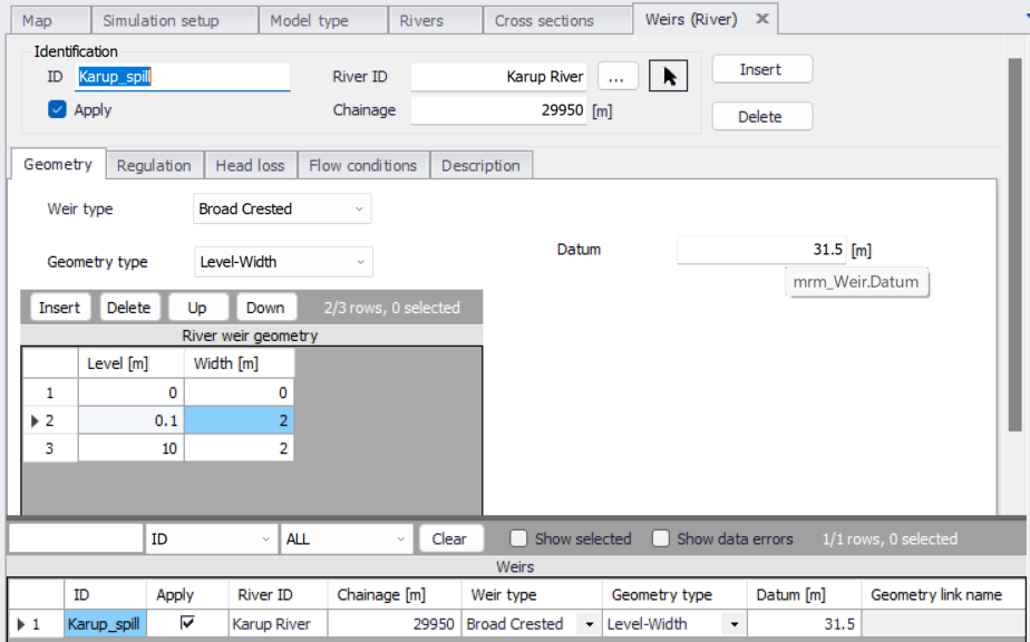
To check the location of the weir in relation to cross sections go to the Map view. The location of the weir is shown as a white square.

Further on the right while being at the Geometry tab, you can see a plot with the position of the weir in relation to the closest upstream and downstream cross-sections.

There is a cross-section 50 m below the weir but none upstream of the weir. As survey data is not available upstream of the weir, you can create a copy of the downstream cross section at chainage 30000 and add it upstream of the weir:

First create a backup of the cross sections file (.xns11), rename it as Karup_basic2weir.xns11 and load this file in the model (browse for it at the Cross sections editor at the General tab.

Go to River network -> Cross sections and right click on the cross section in Map view

Select copy and specify a chainage of 29900

Then, save the setup

Go back to the Weirs editor and select the Flow conditions tab

Click Calculate Q/h relations

Re-run the model

To look at the effects of the weir the model will need to be re-run and the results loaded into Mike View.

Please note that structures generally require smaller time steps so that the model is not affected by instabilities due to exceedances of the Courant number. Therefore, in this case you need to adjust the river model time step (Simulation specifications -> Simulation setup -> HD tab -> Fixed: 30 sec (from 300 sec), and then export and reload in MIKE+ the .m1dx file

To quickly see the effects of the weir, run MIKE+ Rivers with the inflow boundaries changed, as explained previously.

If everything looks fine, run the model in MIKE SHE as before. Remember to change the names of the MIKE SHE and/or MIKE+ Rivers file if you want to keep your old results.

Re-open Mike View and load the results

Click and select Karup River. Press the Ctrl key and click in the view to complete the cross sectional plot. Select Data type = Water level

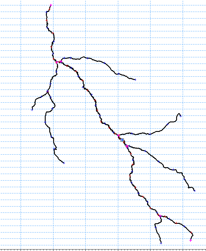
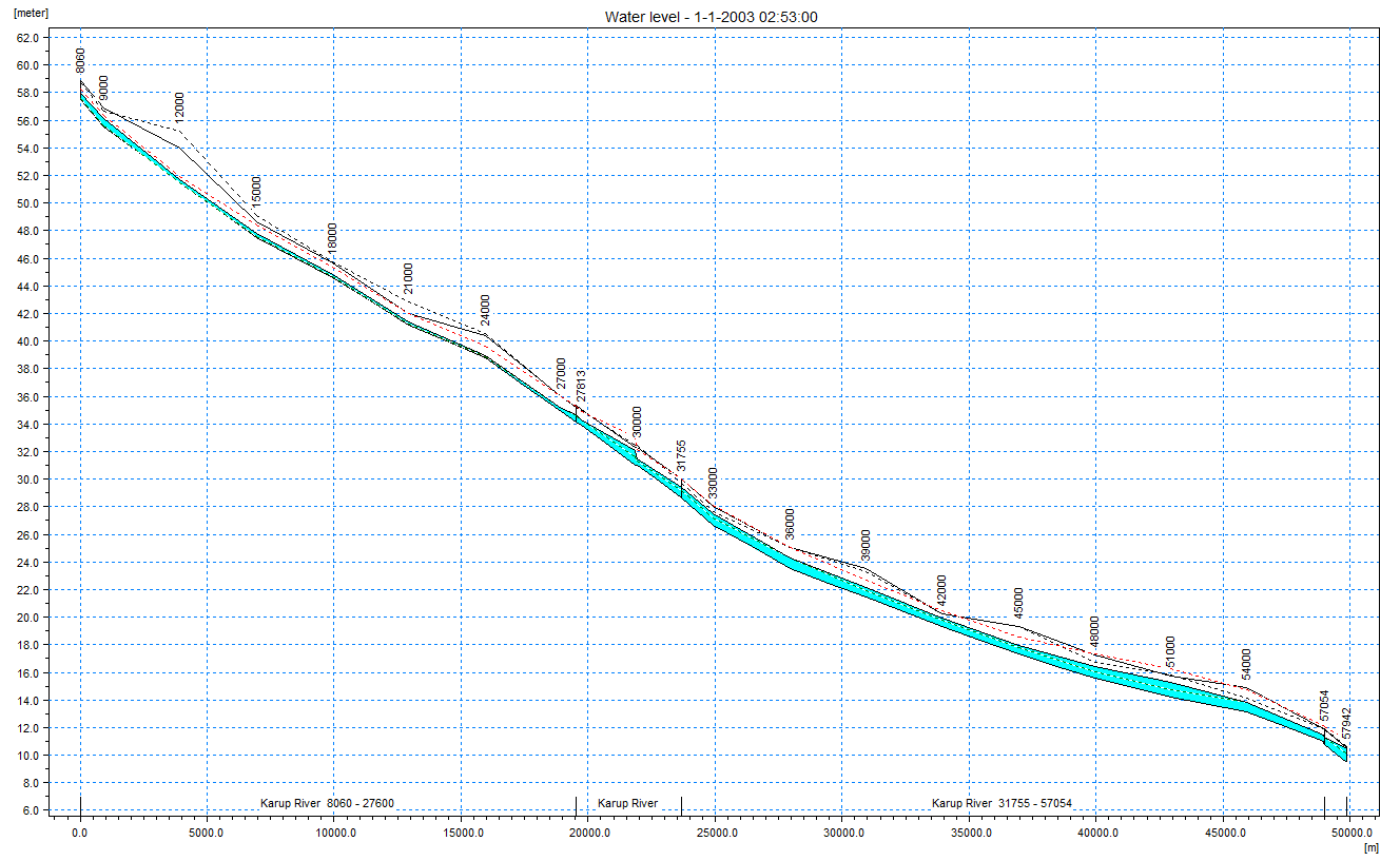
Application Example: Impact of Groundwater Pumping

This exercise shows how groundwater pumping affects groundwater levels and stream flow. The model is based on the MIKE SHE model for Karup developed in the first exercise. If you have completed the first exercise, you can use your own model.

Otherwise, if you want to use an existing model, ensure that you have installed the Example files in the previous Getting Started exercise, and have opened the MIKE SHE exercises.mzp project file. Then,

Go to the project folder Karup_Basic and open Karup_basic.she

In either case,

Rename and save the model using the File/Save As… command to another name (e.g. Karup_basic_250m.she). From now on in the exercise, we will refer to this model as YourFilename.she

Set up a new base case scenario

First, we need to setup and run a new model without groundwater pumping so we can compare the results when we turn on the pumping.

Redefine the horizontal grid resolution

To analyse the effects of an abstraction we need to refine the grid.

A very powerful feature of MIKE SHE is that you can change the horizontal grid without redefining your model parameters. Consequently you can perform sensitivity analysis of your model grid and grid resolution in a way that is impossible with most other modelling user interfaces.

Note: a finer grid is possible, but the simulation time will increase substantially.

Demo Note: The demo version is restricted to a maximum of 70x70 cells, so you will not be able to pre-process or run the model with the refined grid but can continue with the 1000m grid.

In the Model Domain and Grid Dialog of the Setup tab:

Double the number of grid cells in the X and Y directions

Set NX = 130 and NY = 164

Change the Cell Size to 250 m

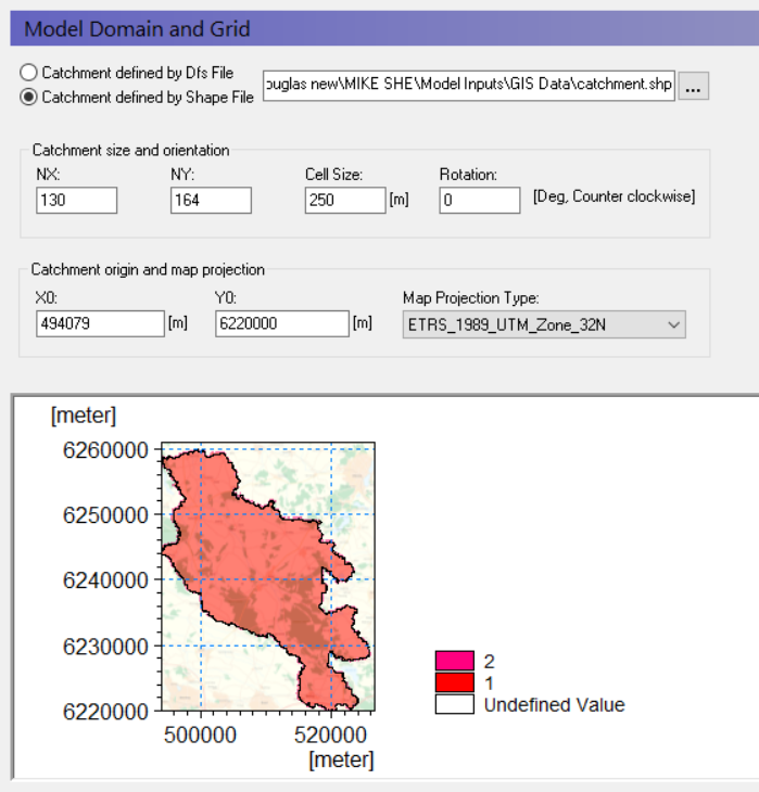
To ensure the model data can be converted to 250 m click on the icon on the main menu to start the pre-processor.

Verify in the pre-processor tab that all of the input data has been converted to a 250m grid

!!! note Notea number of warnings may appear as values are missing in some locations along the boundary. The pre-processor automatically fills in the gaps with neighbouring values.

Add a new stream flow observation

Add a new stream observation location so that you can observe the impact of abstraction on the local stream flow.

Go to Storing of results on the left pane and select Detailed River Timeseries output

Click the add button to add a new line

Specify the Name= Q Pindsobro and change the Data type to Discharge

Type in the Branch name=Karup River and set the Chainage to 15000 m

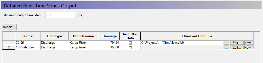
The specified Chainage needs to be at or close to the location of a MIKE+ Rivers computational discharge point. The pre-processor will check the distance and if it is greater than a prescribed tolerance a Warning will be written in the log file.

Add a new groundwater observation

Add a new groundwater observation location so that you can observe the impact of abstraction on the local groundwater level.

Go to Storing of results on the left pane and select Detailed WM timeseries output

Click the add button to add a new line

Specify the Name= Obh_Pindsobro and change the Data type to Head elevation in saturated zone

Type in the coordinates X=513950 and Y=6230800 and Depth=5 m

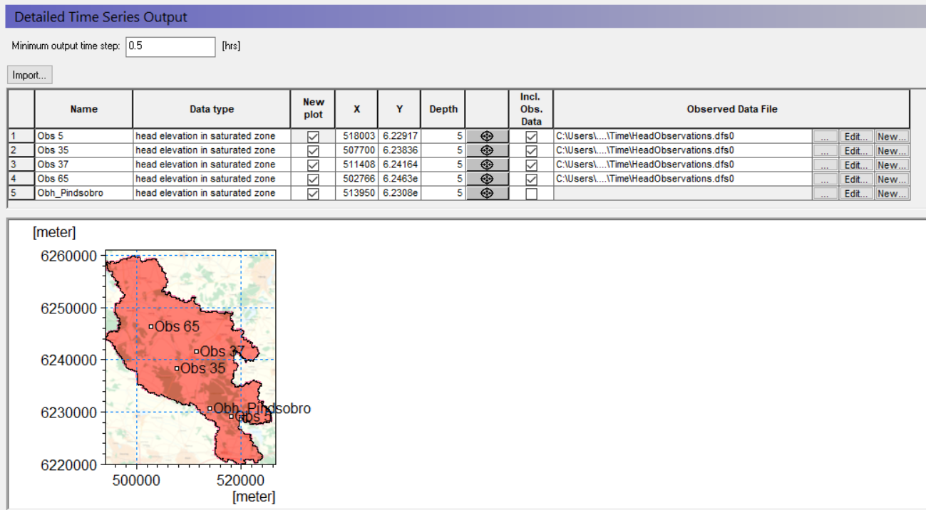
Run the simulation

For this example the simulation period will be reduced to one year, as run times will otherwise be too long:

In the Simulation period menu specify the Start date and End date:

• Start Date: 1 January 2000

End Date: 31 December 2000

On the Toolbar, click on the icon to re-run the Pre-processor and then on the Water Movement icon to run the simulation or just clieck on the Execute icon.

• Click OK

Note if the simulation is taking too long it can be stopped by clicking the red button below.

Check the model run log files to ensure that the model finished without any errors.

Go to the results folder Result\Yourfilename.she - Result Files and double click on YourFilename_WM_Print.log

Scroll to the bottom of the file and check whether the different model components converged. Likely some of the components will have exceeded the maximum number of iterations. The impact of this can be evaluated later with the water balance tool.

Check the stream flow and observation borehole time series plots

After successfully running the model:

Click on the Results Tab located at the bottom of the Navigation Tree and select Simulation Results -> Detailed River Time Series

Click Plot no. 2 to ensure the stream flow plot has been generated and looks reasonable

Do the same for the groundwater observation borehole:

Click on the Results Tab located at the bottom of the Navigation Tree and select Simulation Results -> Detailed WM Time Series

Click Plot no. 5 to ensure the observation borehole plot has been generated and looks reasonable

Create a pumping scenario

Before adding the pumping well, you need to create another scenario setup so that the model results can be compared.

Rename and save the model using the Save As… command: YourFilename_abs.she

The river results will also change, so we also want to create another MIKE+ Rivers setup:

Go to the MIKE+ GUI and load the Karup_basic.mupp project file.

Click File -> Save as.. on the main menu and save the file e.g. as Karup_basic_250m_abs.mupp

Click File -> Export -> Export to m1dx file

Go back to the MIKE SHE Rivers and Lakes menu and use the browse button to select the new file

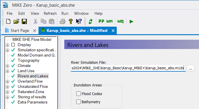
On the Toolbar, click on the icon to re-run the Pre-processor to ensure that the model setup is correct.

Add the groundwater abstraction

In this step, use the Well Editor to add a well beside the stream.

First go to the Saturated zone data tree item to include abstractions and tick Include pumping wells

A new item in the data tree, Pumping Wells, will now appear below Drainage.

Select Pumping Wells and click the button to create a new well database file. This will open the Well Editor in a new window

Browse to the folder .\Model Inputs and name the file e.g. MyWells.wel. Click Save

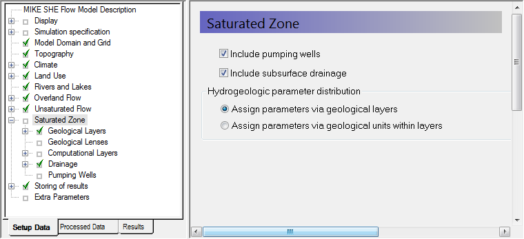
To open the database file click . This will open a new window with the empty database file

The new file automatically shows a map of the catchment outline and the background map specified in the Display menu. The overlays are carried over from the model Setup Tab. You cannot add or modify overlays directly in the Well Editor. This must be done from the Setup Tab. Right clicking on the map, allows you to control the zoom and a number of other functions. The interactive map displays all of the wells in the well file. Clicking on individual wells will select the corresponding item in the table of well locations. Similarly, selecting an item from the list will change the icon of the well on the map to a red square.

To add a new well,

• Click the button to add a new line under Well locations. Then update the line:
• Name = Pindsobro
• Xcoor = 513900,
• Ycoor = 6230750,
• Level = 62 m
• Depth = 60 m.

Next, in the Filter table, click the add button and add the filter settings: - Top = 25 m and

Bottom = 15 m

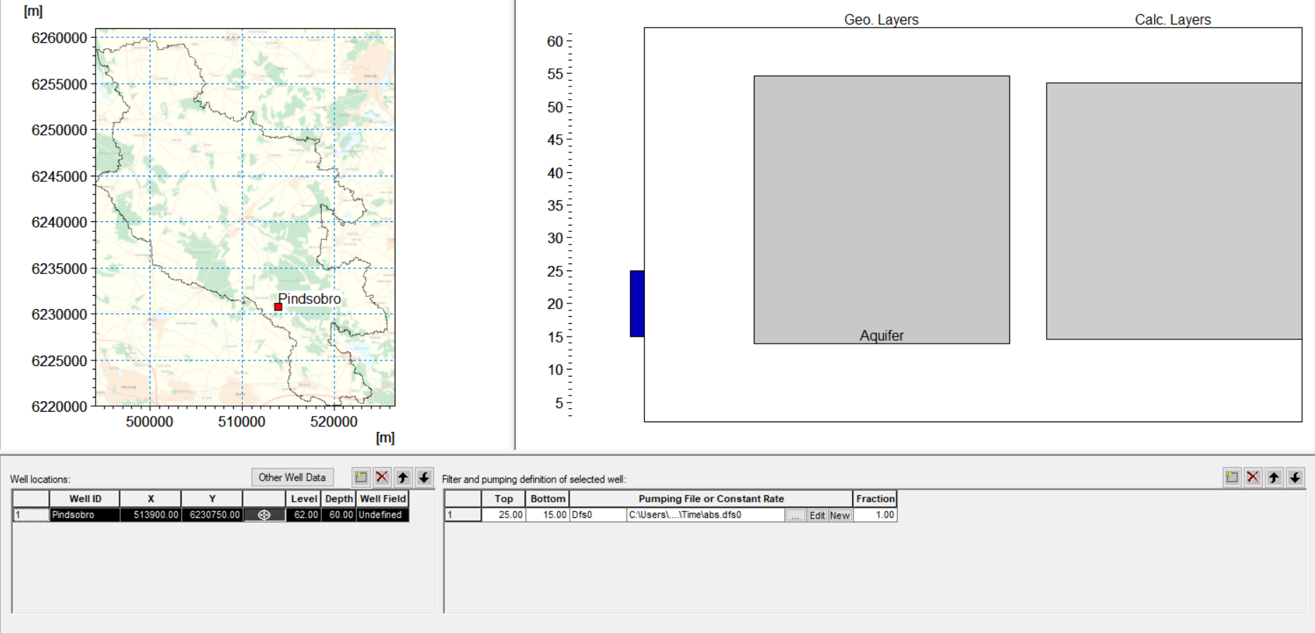
You can see the location of the well on the map view, and the well screen in relation to the geological layers and lenses, as well as the numerical grid layers.

To specify the abstraction rate, click the browse button and select abs.dfs0 and select Item: Pindsobro. Click OK

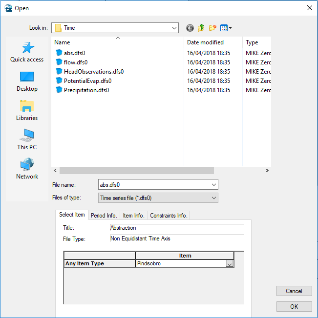
To view the abstraction rate click the edit button . Inspect the .dfs0 file

Close the abstraction time series file

From the Toolbar at the top and Import it also is possible to import well data from a tab delimited ASCII file:

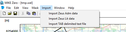
Note: Zeus data is a specialized data format from the Geological Survey of Denmark and Greenland.

Save and close the well file

To view a map showing the location of the abstraction in the MIKE SHE file tick Show well location map

Run the pumping simulation

Before running the simulation, we need to add the results from the original scenario as observations in the pumping scenario.

Add the stream flow result file

To see the difference in stream flow with and without abstraction in the MIKE SHE menu system, add the result file from the model run without the abstraction to the stream plot at Pindsobro:

Go to Storing of results on the left pane and select Detailed River Timeseries Output

On the second line tick Incl. Obs. Data

• Click the browse button and find your detailed time series results for the previous simulation without the abstraction:

YourFilename_DetailedTS_M11.dfs0

Before closing the Selection dialog, under Items select Pindsobro

Click OK

Add the head result file

To see the drawdown caused by the abstraction, you can add the result file from the model run without abstraction to the head elevation plot at Pindsobro.

Go to Storing of results on the left pane and select Detailed WM Time Series Output

On the last line tick Incl. Obs. Data

• Click the browse button and find your detailed time series results for the previous simulation without the abstraction:

YourFilename_DetailedTS_SZ.dfs0

Under Items select Obh_Pindsobro

Click OK

Adding time series of modelled heads from another model run can be done in two different ways, depending on whether observation data is available.

1. In the first case where no observation data is available, you can add the previous results as observations.

Alternatively, you can add a new line below the results item and unclick the New plot checkbox. This way it is possible to add both observation data and multiple simulation results to the same graph. This may be useful during calibration where you want to compare the results from more than one run to the observations.

Run the simulation

On the Toolbar, click on the icon to re-run the Pre-processor and then on the Water Movement icon to run the simulation

When the model is finished, check the log file to ensure the model finished without any errors: YourFilename_abs_WM_Print.log

Analyze the change in stream flow

View the detailed time series output results

To view the stream flow at Pindsobro click on the Results tab at the bottom of the menu and then Simulation Results-> Detailed River Time Series

The black line shows the discharge at Pindsobro for the current model run with the abstraction compared with the results from the model run not including the abstraction (plotted as observation points). It is clear that the abstraction is having a large impact on stream flows all year round due to the vicinity of the well to the stream and high connectivity between the stream and aquifer.

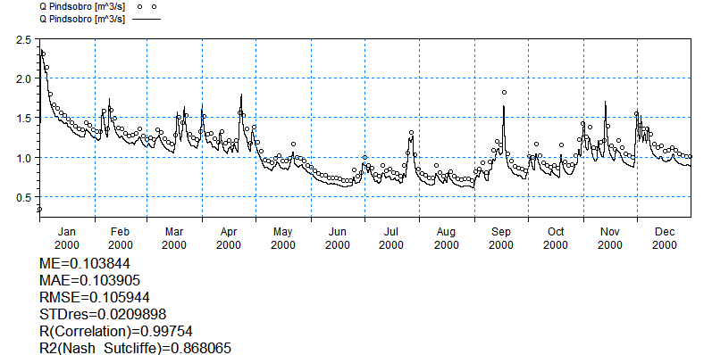
To view the groundwater level close to the Pindsobro abstraction click on go to the Detailed WM Time Series, Plot no 5

The graph shows a significant drawdown in head due to the abstraction.

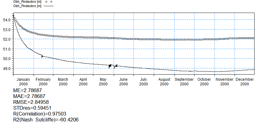
Calculate the difference in the stream flow

To calculate the difference in flow at Pindsobro without and with pumping:

Open the YourFilename_DetailedTS_M11.dfs0 in the results file folder for the refined (250m) model without abstraction:

Click Edit->Properties in the top Menu

Add two new lines to the table by clicking on the button and update the new lines as follows:

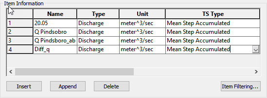
Click OK

From the top Menu, use File->Save as.. and save the file as Q_diff.dfs0

Now,

Open the YourFilename_abs_Detailed_TS_M11.dfs0 in the results file folder for the refined (250m) model with abstraction:

Select the second column named Pindsobro and copy the data to the clip board (\^C)

Return to your Q_diff.dfs0 file and paste (\^V) the data in the third column

Save the file

Now, you need to use the functions option in the Time Series Editor to calculate the difference in flow between the two columns:

click on the toolbar at the top

Type in the Current Expression textbox: i4=i2-i3

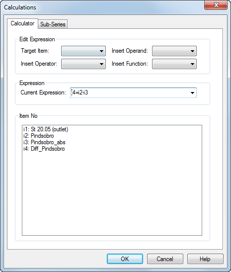
Click OK and save file

This should immediately fill in the fourth column with the difference between Column 2 and 3.

Use the Plot Composer to plot the impact on stream flow

To plot the flows and the differences using the Plot Composer tool:

Create a new Plot Composer document from File/New in the top menu or use the New File icon, and then select the Plot Composer icon in the list of MIKE Zero documents.

Insert a new plot using either Plot->Insert New Plot Object and select Time Series Plot or by clicking on the New Plot icon, , and selecting the Time Series Plot

In the Properties dialog that appears, click New Item and select your Q_diff.dfs0 from the list

Under Any Item Type select Q Pindsobro, Q Pindsobro_abs and Diff_q

Click OK

To change the appearance of the graphs, right click on the graphs and select Properties. Click Curves and change line colours and markers

To save the graph as an image click View->Export Graphics->Save to Bitmap

Save the plot composer file as Q_diff.plc in the Model folder

You should get a plot looking something like this:

Use MIKE View to calculate the change in stream flow accretion

We want to look at the effect of the pumping on stream flow accretion along the Karup River at different times. To do this:

Use Windows Explorer to navigate to the results folder for the MIKE+ Rivers simulation with abstraction, and then double click on the file: Karup_basic_1BaseDefault_Network_HD.res1d that is located within the Karup_basic_250m_abs_m1d - Result Files folder

Click OK to load all the data

This should open the MIKE+ Rivers result file in MIKE View. If for some reason this does not work, you can also open MIKE View from the Program menu and load the file. If the file is not yet loaded,

• add the MIKE+ Rivers result file (*.res1d) abstraction to MIKE View using the File/Add in the top menu.
• Click OK to load the result file

Once MIKE View is open, with the results loaded, we want to plot the stream flow accretion with and without pumping. To do this:

Click the profile button on the main menu to draw a profile

Click on the middle branch of Karup stream (the branch turns green), press the Ctrl key, click in the view, and select ‘Yes’ to create the longitudinal plot.

Select Data Type=Discharge, and click OK

Now, to add the no-pumping MIKE+ Rivers *.res1D

Go back in the main window, choose File and click Add. Now navigate to your no-pumping result file.

Click on the longitudinal profile window and click on the Options icon

Select the Graphical Items tab

Click the Add button . Then select Dynamic Item, File= Karup.res1d (your file without pumping) and Item=Discharge. Then click OK.

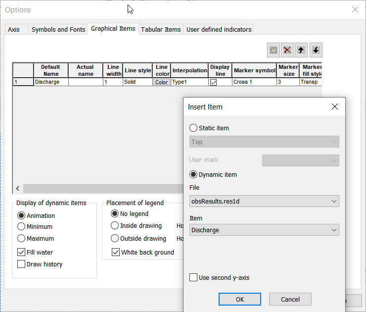
You may want to chose a different line colour etc, change the Actual name, etc. Then click OK

Note that you may have press the play button to see the plot.

To save the plot layout, right-click on the map view and select Save complete layout.

Save the file as Stream_flow_acc.CLA

You can then reload this file in future to recreate the plot.

To re-load the file click File->Reload complete layout…and select Stream_flow_acc.CLA located in .\Result

Click OK and OK to load the MIKE+ Rivers result files

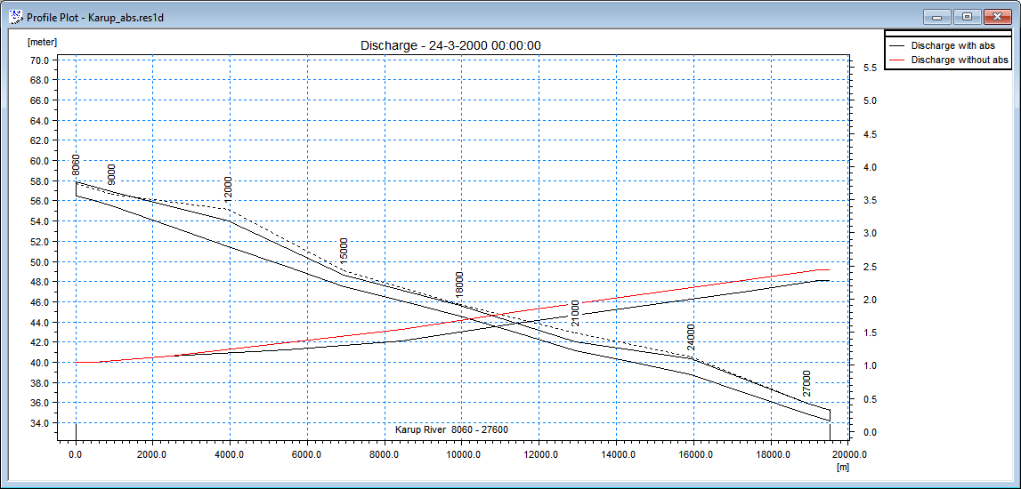
Analyze the well drawdown

To evaluate the radius of influence of the well, we can look at the well drawdown in space and time. To do this we need to subtract the no-pumping results from the pumping results. There are basically two ways to do this.

Grid Editor - The most direct way is to subtract the files from within the Grid Editor

Grid Calculator - However, if you want to do this regularly, say at the end of every simulation you can set up a script using the Grid Calculator Tool in the MIKE SHE Toolbox.

Calculate drawdown using the Grid Editor

To calculate the difference in groundwater levels at Pindsobro without and with pumping:

Open the YourFilename_3DSZ.dfs3 with pumping in your Results directory, and save the file to a new name (eg DrawdownGridEditor.dfs3) using the File/Save as… menu function.

Demo Note: In Demo mode, you will not be able to save any changes to the dfs3 file.

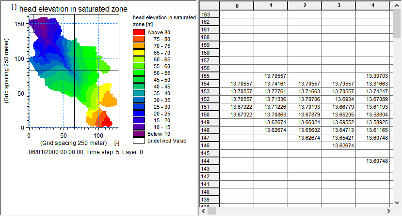
Now, to subtract the two results files:

Click Tools->Copy File into Data on the main menu

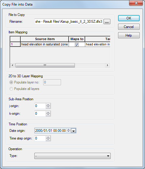
Select the File to Copy using the browse button , and find your no-pumping _3DSZ.dfs3 results file

Under Operation Type: choose the minus sign, “–“

Click OK, and then Yes to continue

This process will change every value in every time step, by subtracting the two values. The result will be a dfs3 containing only the differences.

You can view the new values by

Clicking on the Time Step Forward and Backwards buttons to view the drawdown at different times

Zoom in by right clicking on the map

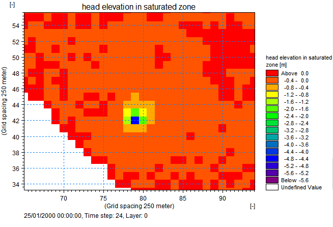
MIKE SHE includes sophisticated tools for managing gridded data as well as time series data. This is very useful for time varying distributed parameters, such as precipitation that is interpolated from rain gauge data, or distributed recharge calculated by third party programs.

The grid editor is a split window that can be dragged sideways to make the map smaller or larger. The table of values on the right side reflects the highlighted grid shown on the map.

Ranges of values can be searched for, selected and changed using the select and unselect tools, , plus the Tools/Set Value… Dialog.

Important Note

The grid editor is a generic grid tool for all DHI Software, and was originally developed for the Marine programs MIKE 21 and MIKE 3. However, this often leads to confusion in the node and layer numbering because MIKE 21 and MIKE 3 use a different numbering system.

Node numbering: In the Grid Editor (and in MIKE 21 and MIKE 3) the nodes are numbered starting in the lower left from (0,0), whereas in the MIKE SHE dialogs and log files the nodes are numbered starting in the lower left from (1,1).

Layer numbering: In the Grid Editor (and in MIKE 21 and MIKE 3) the layers are numbered starting at the bottom from 0, whereas in the MIKE SHE dialogs and log files the layers are numbered starting at the top from 1.

Calculate Drawdown with the Grid Calculator

To make this conversion, you can:

Click on the New File icon, or the File/New/File… top menu. Then select the MIKE SHE toolbox.

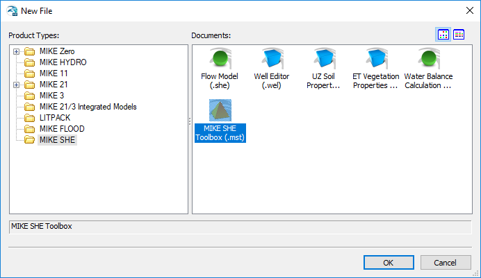
Now select Util/Grid Calculator

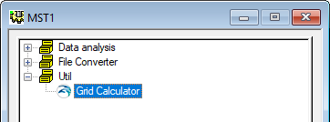
Add a title if you want and then click

In the Calculation Setup dialog that appears:

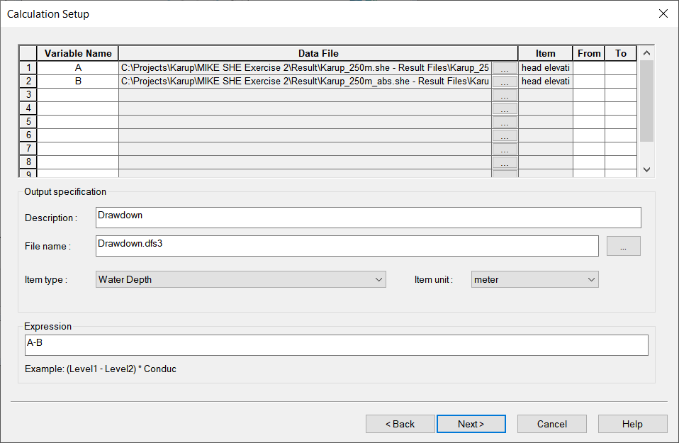
Browse to the two dfs3 head results files (pumping and no pumping) and add them to the list of items with a Variable name of A and B.

Add a Description, if you like, and a Filename, such as DrawdownGridCalculator.dfs3

Select the Item type = Water Depth, with Item Unit = meter

Now set up the Expression “A-B”. Note that the variable names are case sensitive

Then, click

On the last page, click to run the actual conversion

Click OK in the window saying successful completion

Click to close the tool.

The Grid Calculator is a very useful tool. It allows you to do complex, multi-step, operations on files. It also has limited statistical functions, as well as a Group function. Together these allow you to create sophisticated analyses, such as the minimum monthly water levels over your simulation, or the number of days that are area is flooded per year.

You can also save the Toolbox tool and run it at the end of your simulation. You can also run the Grid Calculator from a command prompt or batch file directly.

Plot the drawdown using the Plot Composer

You can look at the drawdown in the Grid Editor, but if you want to create a report plot, you can use Plot Composer.

However, the Plot Composer does not support dfs3 files. Therefore, first you need to convert the drawdown file from a .dfs3 file to a .dfs2 file. To make this conversion, you can:

Click on the New File icon, or the File/New/File… top menu. Then select the MIKE ZERO toolbox

Now select Extraction/2D Grid from 3D files

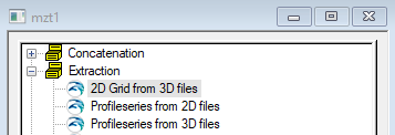
Add a title if you want and then click

Browse to your DrawdownGridEditor.dfs3 file and click

Click again for all time steps, and click again for the default layer

Specify a File Name and Title for the output file (eg DrawdownGridEditor.dfs2). Then, click

On the last page, click to run the actual conversion.

Click OK in the window saying successful completion

Click to close the tool.

If you save the tool setup, then you can run it again without having to update it. You can also run a saved toolbox setup from a batch file.

Now open a new Plot Composer document to create a drawdown map as you did before.

Click Plot->Insert New Plot Object and select Grid Plot

In the Grid Plot Properties menu select the Master File as DrawdownGridEditor.dfs2

Select the Contours menu

Tick With labels and tick Plot color Legend

Click OK

To view the drawdown at different times first select the Animate menu at the bottom left

Use the play menu to move through the file

To change the colours or layout go back to the menu and right click on the map. Select Properties. Play with the colour scale.

To add the stream to the map right click on the map and select Add/Remove layers….

Click the add button to add a new item

Change File type to Shapefile and in .\Model Inputs\GIS data select Karup_system.shp

Click

To save the graph as an image click View->Export Graphics->Save to Bitmap

Click File->Save as.. and save the file as Drawdown.plc

Analyze the change in water balance

You can use the water balance tool to look at the impact of the abstraction.

Create a new water balance document

Click on the New document icon, , or the File/New/File menu

Select MIKE SHE and then the Water Balance Calculation (.wbl) document

Click OK

Then go to File menu -> Save as to save within the folder Karup_basic_250m_abs.she - Result Files and give the file a name (e.g. Wbl_abs)

Extract the water balance data

Use the browse button and find the .sheres file from your simulation in your Result directory

Run the water balance extraction by clicking on the Extraction icon, or by selecting the drop down window Run and clicking on Extraction.

Check to make sure that the Extraction ran successfully, by looking for “Normal termination” in the message window

Define a Chart water balance

As there will only be only item it is not ncessary to add more items on the Postprocessing tab

Select Chart output: Total water balance from the list of available Water balance types.

Define a file name for the output file, for example Water_balance_abs.txt

Run the water balance by clicking on the water balance icon run selected postprocessing,

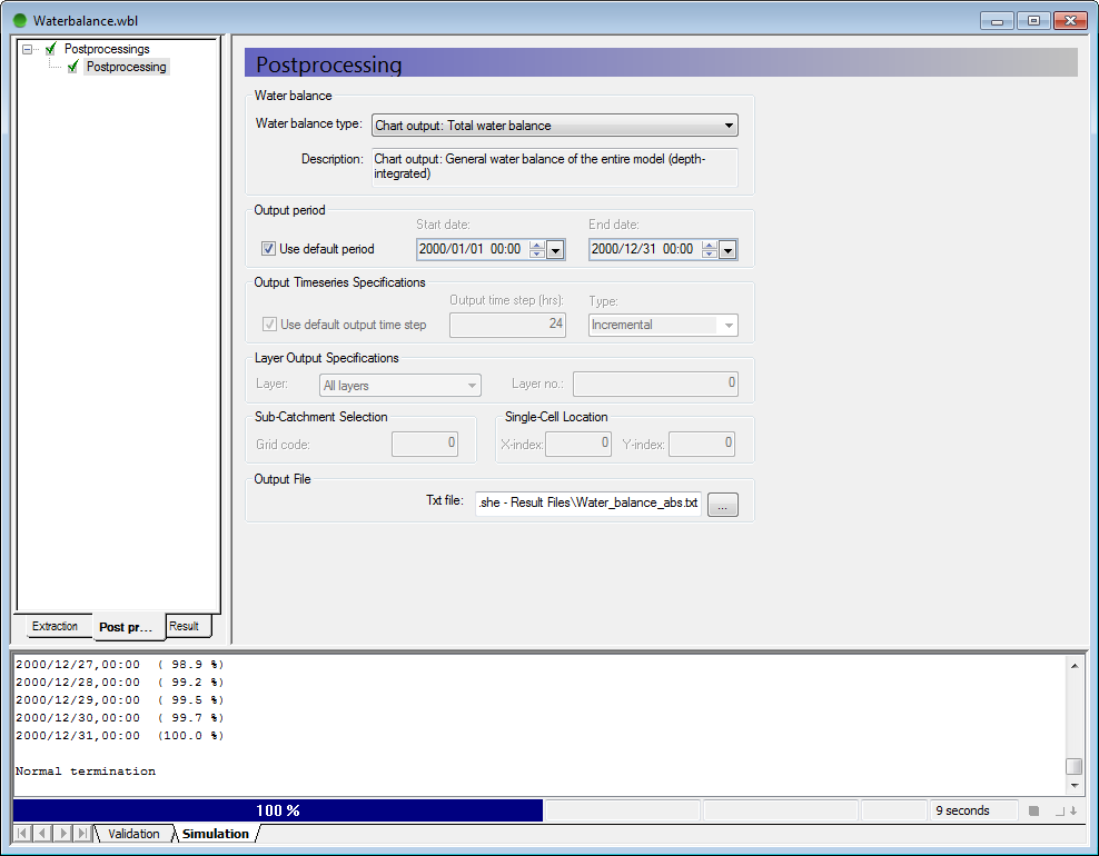
The Chart output creates a graphic illustrating the water balance items (see next step). The output is sent to an ASCII .txt file, and the graphic is generated automatically by a utility that reads the txt file.

By default, the water balance is summed for the entire simulation period. However, you can easily change the water balance period, for example, to create seasonal water balances, or to remove the initialisation period.

If you defined the extraction on a sub-catchment basis, then you can select from the available sub-catchments in this Dialog.

View the water balance output

On the Result tab, select the sub-item for the Chart output

Click on the Open button beside the file path to create and open the water balance graphic

To compare the water balance with abstraction to that without abstraction repeat the same procedure for the model run without abstraction

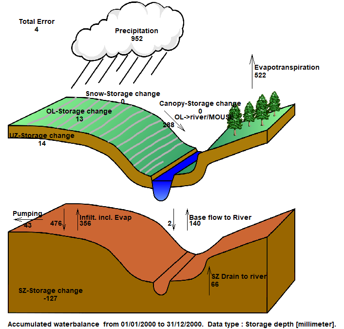
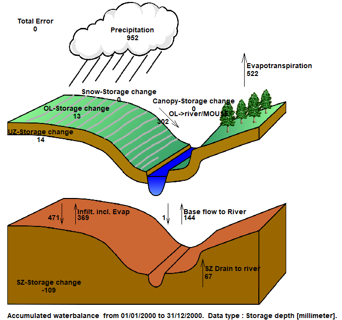
The water balances show that during the simulation period a total of 43 mm is abstracted.

Additional optional exercise: Play around with the different water balance options to see how baseflow, drain flow and saturated zone storage may be changing over time due to abstraction.

augNote that the water balance items are all normalised to units of mm, which allows for easy comparison between the different components. If you want to convert depths of mm to volumes, you need to multiply the depth by the internal model area. That is, the total model area minus the area of the outer boundary cells.

An easy way to calculate the internal model area is to load the pre-processed data into the Grid Editor, select the Model and Domain item. Then, you can use the statistics function in the Grid Editor to find out the number of internal (Grid Code = 1) versus boundary cells (Grid Code = 2).

Application Example: Convert to a Rainfall-Runoff model

This exercise shows how to convert the Karup model to a simple rainfall-runoff model that uses the Linear Reservoir SZ and the Simple 2-Layer UZ methods. This model would be suitable to run with the MIKE SHE Studio version.

Create a copy of an existing Karup model

To start this exercise, you can use either your basic Karup setup that you created, or you can use the pre-defined Karup_basic.she model. In either case, make sure to create a copy of the .she model that you are going to use. Then, open the new .she model.

Change the numerical methods

The first thing to do is to change the numerical methods for the UZ and SZ model in the simulation specification.

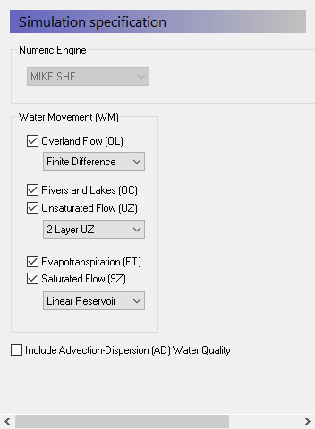
Set the UZ method to the 2 Layer UZ and the SZ method to Linear Reservoir

This will change the data tree:

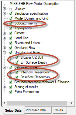
You will see six new entries in the tree:

• Subcatchments – these are the catchment areas for each major stream branch where you want to separate the flow
• 2 Layer UZ Soil – this is the soil distribution
• ET Surface Depth – this is the thickness of the capillary zone for the UZ soils
• Interflow Reservoirs – these are the shallow, short duration groundwater storages
• Baseflow Reservoirs – these are the deeper, long duration groundwater storages

Groundwater table for lower UZ boundary: this is used to define the thickness of the unsaturated zone.

Define the subcatchments

The subcatchments define the discharge areas for the Interflow reservoirs. In this exercise we will use a single subcatchment.

Set the Spatial distribution to Uniform

In the sub-tree item, there is only one option: Use default river links. This option is useful in real models where you have a complex distribution of subcatchments. Also, the stream discharge is uniformly distributed to the branches. This option allows you to be sure that the water discharges to a specific reach.

Define the 2 Layer UZ model

This is in the Unsaturated Flow data tree item. In the 2-Layer UZ soil, use the Distributed option and then use the same soils distribution file as in the original Karup model.

Browse to the Model Inputs\Maps\soils.dfs2

Then, for each soil use the appropriate soil properties from the UNSODA soils database file.

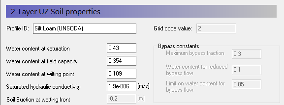
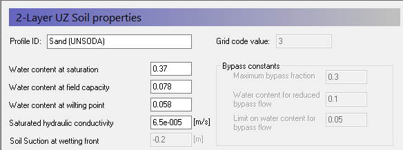
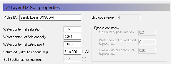
The ET Surface Depth is the thickness of the capillary fringe. The default value is 0.1m. For sandy soils this is probably suitable, but for finer soils it should be thicker.

The ET Surface Depth is used to extract ET directly from the groundwater table. if the groundwater table is close to the bottom of the root zone.

However, in this exercise, the Linear Reservoir method does not calculate a water table, Thus, this depth is not used unless the predefined SZ static water table is close to the Root Zone, so you can leave it at the default value.

Define the Linear Reservoir groundwater model

Define the Interflow reservoirs

The interflow reservoirs are used to define the quick stream flow response after a rainfall event. The interflow reservoirs have two outlets – one to the downgradient interflow reservoir or stream, and one to the underlying baseflow reservoir.

If you have multiple interflow reservoirs, the higher number reservoir discharges “downhill” into the lower number reservoir. Thus, the interflow reservoirs are essentially, topographic zones around the streams. The lowest Interflow reservoir discharges to the stream.

The Interflow reservoirs discharge into the streams branches within the subcatchment. Typically, you will have multiple subcatchments – often with the subcatchments and interflow reservoirs being the same.

In this exercise, we will use a single interflow reservoir. However, in most models this would not be the case.

• Set the Spatial distribution to Uniform
• Set the Specific Yield to 0.129, which is a representative value for the predominant soil.

Leave the rest of the default parameters for now.

Define the Baseflow reservoirs

The Baseflow reservoirs represent the slow groundwater discharge to streams. The Baseflow reservoirs have only a single outlet – the stream.

By default the discharge from the baseflow reservoir is evenly distributed to all stream nodes in the model. The “Use default river links” allows you to define where the baseflow should be discharged.

In large catchments you may have several baseflow reservoirs representing large subcatchments. In this exercise, we will use a single baseflow reservoir.

The two baseflow reservoirs act in parallel. Typically, one will have a longer time constant than the other. This allows you to capture the slow drainage after a storm, as well as the dry season flow. The Fraction of percolation to Reservoir 1, allows you to distribute the amount of water percolating from the Interflow reservoirs to each of the two Baseflow reservoirs.

• Set the Spatial distribution to Uniform
• Set the Specific Yield in both reservoirs to 0.129, which is a representative value for the predominant soil.

Leave the rest of the default parameters for now.

Define the UZ lower boundary depth

The UZ lower boundary is defined by the water table. However, the Linear Reservoir SZ does not calculate a water table. Thus, you need to define the water table depth for the UZ lower boundary.

• Set the Spatial distribution to Uniform
• Set the depth to -3 m, and

Ensure that the Values relative to ground is checked on

Calibrate the model

On the Toolbar, click on the icon to re-run the Pre-processor and then on the Water Movement icon to run the simulation

Evaluate the results and calibrate the model

You will see that the discharge results are not very good. The Linear Reservoir method is quite easy to calibrate, if you understand how the different parameters affect the discharge.

Essentially,

• The time constants affect the rate of discharge from the reservoirs. You can adjust the various time constants to match the shape of the observed discharge hydrograph.
• The initial depth governs the initial discharge rate. Usually, the Interflow reservoirs are started dry. That is the initial depth equals the bottom depth. The Baseflow reservoirs usually start with a small amount of water.
• The threshold depth allows you to have storage that does not discharge to the stream. In the Interflow reservoirs, water below the threshold will still percolate to the Baseflow reservoir. In the Baseflow reservoirs, water below the threshold can still be pumped.
• The UZ fraction allows some of the water to be added to ET instead of the stream

The Dead Zone storage allows some of the percolation to be “lost” and not available for discharge.

The default values for the time constants do not give very good results. You can play with these values to see how they affect the hydrograph.

After playing with the values you can try the following values which give a reasonable calibration:

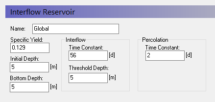
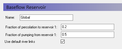
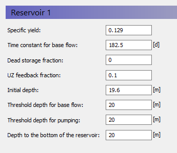
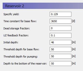
Evaluate the water balance

When you compare the water balance with the original model, you will see quite big differences, for instance in the baseflow to the river and the infiltration. The first water balance below is for the original model, while the second is for the Rainfall-Runoff model.