Simplified Overland Flow Routing
The conceptual reservoir representation of overland flow in MIKE SHE is based on an empirical relation between flow depth and surface detention, together with the Manning equation describing the discharge under turbulent flow conditions (Crawford and Linsley, 1966). This was implemented in the Standford watershed model and in its descendants, such as HSPF (Donigian et al., 1995), and has been applied in other codes such as the WATBAL model (Knudsen, J. 1985a; Knudsen, J. 1985b;Refsgaard and Knudsen, 1996).
In the following, a description of the principles behind the model and the governing equations implemented and solved in MIKE SHE are presented. It is implicitly assumed that the equations derived for a hill slope can be applied to describe overland flow, in a lumped manner, across a catchment.
1. Theoretical basis
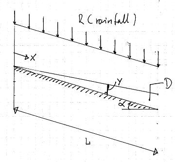
Figure 29.8 Schematic of overland flow on a plane
Figure 29.8 represents a schematic of overland flow on a planar surface of infinite width with uniform rainfall. Precipitation falls on the plane, builds on the surface in response to the surface roughness, and flows down the slope in the positive x-direction. In the figure, L is the length of the slope, y is the local depth of water on the surface at any point along the surface and \(\alpha\) is the slope. Then, from the continuity equation
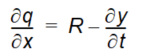
Equation 29.41
where
- q is the specific discharge.
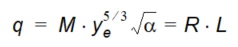
For turbulent flow on a plane of infinite width, the Manning equation is
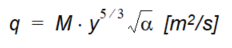
Equation 29.42
where
- q is the specific discharge
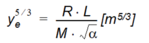
Now, at equilibrium, the depth no longer changes and the specific discharge approaches the rainfall rate
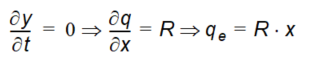
Equation 29.43
where
- q is the specific discharge.
- qe is the equilibrium specific discharge.
Then, at equilibrium, the volume of water detained on the surface, De, can be calculated by
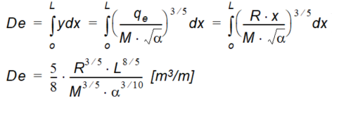
Equation 29.44
where
- q is the specific discharge
The depth, y, near the leading edge of the flow plane can be related to the depth at equilibrium by
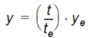
Equation 29.45
where
- q is the specific discharge
where
- t is the time
- te is the time until the equilibrium is reached. Then from (29.42) we can write
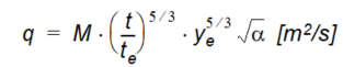
Equation 29.46
where
- q is the specific discharge
Now if we integrated the specific discharge from time 0 to when the equilibrium is reached, we can calculate the total volume discharged, Q, (per unit width of the plane) by
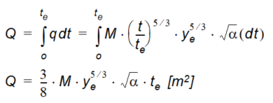
Equation 29.47
where
- q is the specific discharge
From (29.46), at equilibrium, (t = te), the depth of water at the leading edge of the plane (x = L) is
Equation 29.48
where
- q is the specific discharge.
Equation 29.49
where
- q is the specific discharge.
From continuity, the total volume of inflow up until equilibrium must equal the total outflow minus the amount retained on the surface. Thus,
Inflow - Outflow = Surface storage
which from equations (29.47) and (29.44) yields
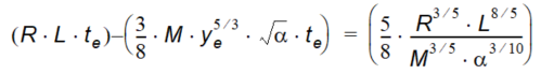
Equation 29.50
which, when simplified, yields the time to reach equilibrium

Equation 29.51
If we now assume that the flow on the sloping plane is uniform, that is the change in discharge as a function of x is zero, then the depth prior to equilibrium is simply

Equation 29.52
and the relationship between the depth, y, and the surface storage at equilibrium, De, is given by
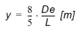
Equation 29.53
The relationship between the depth, y, and the detained surface storage prior to equilibrium, D, is given by an empirical model (Fleming, 1975; Crawford and Linsley, 1966)
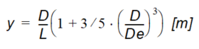
Equation 29.54
where during the recession part of the hydrograph, when D/De is greater than 1, D/De is assumed to be equal to 1.
Substituting (29.54) into the Manning equation (29.42) yields
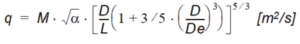
Equation 29.55
Implementation in MIKE SHE
In MIKE SHE the current level of surface detention storage is continually estimated by solving the continuity equation
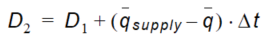
Equation 29.56
where
- D1 is the detained storage volume at the start of the time step and D2 is the detained storage volume at the end of the time step
- q is the overland flow during the time interval
- qsupply is the amount of water being added to overland flow during the time step. Since q is a function of the average detained storage volume, (D1+D2)/2, equation (29.55) is solved iteratively until a solution satisfies both equations.
2. Coupling to other processes
Overland flow interacts with the other process components, such as evapotranspiration from the water surface, infiltration into the underlying soils, interaction with soil drains, drainage into the channel network, etc. This is an integral part of the MIKE SHE framework and these interactions are treated in the same manner in both the Semi-distributed Overland Flow Routing model and the 2D Finite Difference Method, based on the diffusive wave approximation.
The Semi-distributed Overland Flow Routing model simulates flow down a hillslope. To apply this at the catchment scale, it is assumed that the overland flow response for a catchment is similar to that of an equivalent hillslope. Furthermore, the drainage of overland flow from one catchment to the next, and from the catchment to the river channels is represented conceptually as a cascade of overland flow reservoirs.
3. Avoiding the redistribution of ponded water
In the standard version of the Simplified Overland Flow solver, the solver calculates a mean water depth for the entire flow zone using the available overland water from all of the cells in the flow zone. During the Overland flow time step, ET and infiltration are calculated for each cell and lateral flows to and from the zone are calculated. At the end of the time step, a new. average water depth is calculated, which is assigned to all cells in the flow zone.
In practice, this results in a redistribution of water from cells with ponded water (e.g. due to high rainfall or low infiltration) to the rest of the flow zone where cells potentially have a higher infiltration capacity. To avoid this redistribution, an option has been added where the solver only calculates overland flow for the cells that can potentially produce runoff, that is, only in the cells for which the water depth exceeds the detention storage depth.
Example application
To illustrate the effect of this option, it was applied to a model with a 10 x 10 square domain, one subcatchment and 3 different soil types in the unsaturated zone with the following saturated hydraulic conductivities
- coarse1e-5 m/s
- medium 1e-7 m/s
- fine 1e-9 m/s
For rainfall, a synthetic time series with alternating daily values of 50 and 0 mm/day was used. The simulation period was 2 weeks. Thus, the cumulative rainfall input was 350 mm.
For the case, where the ponding water was not redistributed, the cumulative runoff was 96 mm. Whereas, when the ponded water was redistributed, the cumulative runoff was essentially zero.
Activating the option
This option is activated by means of the boolean Extra Parameter, Only Simple OL from ponded, set to On. For more information on the use of extra parameters, see Extra Parameters.
4. Routing simple overland flow directly to the river
In the standard version of the Simplified Overland Flow solver, the water is routed from 'higher' zones to 'lower' zones within a subcatchment. Thus, overland flow generated in the upper zone is routed to the next lowest flow zone based on the integer code values of the two zones. In other words, at the beginning of the time step the overland flow leaving the upper zone (calculated in the previous time step) is distributed evenly across all of the cells in the receiving zone. In practice, this results in a distribution of water from cells in the upstream zone with ponded water (e.g. due to high rainfall or low infiltration) to all of the cells in the downstream zone with potentially a large number of those cells having a higher infiltration capacity. In this case, then, overland flow generated in the upper flow zone may never reach the stream network because it is distributed thinly across the entire downstream zone.
To avoid excess infiltration or evaporation in the downstream zone, an option was added that allows you to route overland flow directly to the stream network. In this case, overland flow generated in any of the overland flow zones is not distributed across the downstream zone, but rather it is added directly to the river stream network as lateral inflow.
Example application
To illustrate the effect of this option, it was applied to a model with a 10 x 10 square domain, one subcatchment and two overland flow zones. The upper zone included an unsaturated zone with a low infiltration capacity, whereas the lower zone had a high infiltration capacity. The saturated hydraulic conductivities of the two zones were
- upper zone 1e-9 m/s
- lower zone 1e-5 m/s
For rainfall, a synthetic time series with alternating daily values of 50 and 0 mm/day was used. The simulation period was 2 weeks. Thus, the cumulative rainfall input was 350 mm.
For the case, where the overland flow was routed directly to the river, the cumulative runoff to the river was 167 mm. Whereas, when the overland flow was routed first to the lower zone, the cumulative runoff reaching the river was only 1 mm.
Activating the option
This option is activated by means of the boolean Extra Parameter, No Simple OL routing, set to On. For more information on the use of extra parameters, see Extra Parameters.