MIKE SHE Toolbox¶

1. Probability curves (*.dfs0)¶

The MIKE SHE Probability Curves Tool calculates the mean value, as well as the probablity and duration curves for the specified period in a dfs0 file

Setup Name¶

Specify a name for the setup. This allows you to save and retrieve the setup, either later, or from a batch file.

Time series file selection¶

Select the dfs0 file for which you want the probablity and duration curves.

Output Settings¶

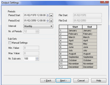
The output settings dialogue allows you to define the period and interval for the statistic calculation. If you select Specified for the Interval, then you can define the number of periods and the start and end months.

The sub-sets option allows you to further refine the statistical breakdown.

Output file selection¶

Type in the name of the ASCII file where want the probability and duration curves written to.

Status¶

The Status page presents you with a summary of all the input parameters you have specified. Check that the parameters are correct. If not go back andchange them.

Log/pfs file location

This is the directory where the output will be sent. A subdirectory will be created here based on the name of the setup.

Running the Tool

Finally, on the Status page, you can

Execute the setup, which will run the Tool with the current parameters, or
Finish the setup, which will save your setup definition in the current toolbox file.

The tool runs silently. If there are any errors, then the tool will simply not run.

2. dfs2+dfs0 to dfs0¶

This tool is used to build a time varying dfs2 file from a dfs2 grid code file and one or more dfs0 time series files. The time varying dfs2 file can be used for time varying gridded data items, including Precipitation Rate and Evapotranspiration.

Setup Name¶

Specify a name for the setup. This allows you to save and retrieve the setup, either later, or from a batch file.

Files¶

This dialogue contains the file name for the two input files and the output file.

The input file is a dfs0 file, usually with multiple data items. All the data items are expected to have the same units, but this is not checked.

The input dfs2 file is a grid file with grid codes corresponding to the item numbers in the dfs0 file. The dfs2 file must have an EUM type of Grid Codes with a unit of Integers.

If you are creating a distributed precipitation rate file, then the dfs0 items must be of type “Mean Step Accumulated”, with a EUM Type of Precipitation Rate and any valid unit, such as [inches/hour] or [mm/day].

The output file will be a dfs2 file with one grid for each time step in the dfs0 file. and the values in each grid point equal to the value in the dfs0 file at that time step.

Status¶

The Status page presents you with a summary of all the input parameters you have specified. Check that the parameters are correct. If not go back and change them.

** Log/pfs file location**

This is the directory where the output will be sent. A subdirectory will be created here based on the name of the setup.

Running the Tool

Finally, on the Status page, you can

Execute the setup, which will run the Tool with the current parameters, or
Finish the setup, which will save your setup definition in the current toolbox file.

The tool runs silently. If there are any errors, then the tool will simply not run.

3. Grid Calculator¶

The MIKE SHE Grid Calculator tool allows you to perform complex operations on .dfs2 and dfs3 grid files.

The Grid Calculator tool has been upgraded to handle time varying dfs files with multiple Items. The documentation also now includes examples on how to use the tool from a script.

The only limitation is that all the grid files must have the same grid dimensions and the same number of time steps must be loaded for each item.

a. Setup Name¶

Specify a name for the setup. This allows you to save and retrieve the setup, either later, or from a batch file.

b. Calculation Setup¶

Note

All fields must be filled in.

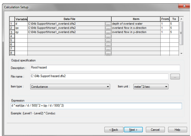
In the first part of the dialogue, you need to specify the files and variable names used in the mathematical operation. These will be the variables used in the subsequent operation.

Note

The variable and function names are case sensitive

Output Specification

In the second part, you must specify the output file name (including the .dfs2 or dfs3 file extension), as well as the EUM unit type and units for the resulting file. Although the EUM list is alphabetical, the list of EUM data types is very long, as it includes all of the available EUM types for all of the MIKE Zero products. If you are trying to create a particular input type for MIKE SHE, then you should look in the MIKE SHE Setup dialogue, to find out first what EUM data type is required and then find this type in the list.

Expressions¶

The last part of the dialogue is the mathematical expression you wish to evaluate. The standard order of operations is followed, including the use of nested brackets.

Operators

Valid operators are: +, -, *, /, and ^.

These (binary) operators can be applied to:

Two scalars (single floating point numbers)
Two arrays of equal structure (e. g. two variables containing data read from two dfs files, where the same spatial and temporal extent has been read from each file). If the two arrays do not match in size, an error will be reported.
An arbitrary array and a scalar. In this case the operation will be performed on each element of the array and the scalar, so the result has the same dimensions and extents as the input array.

Functions with a single argument

Valid functions with a single argument are:

fabs - absolute value
ceil - maximum value in the time series
floor - minimum value in the time series
log, and log10 - natural and base 10 logarithm
sqrt - square root
sin, cos, tan, asin, acos, atan - trigonometry functions

These functions can be applied to any array or scalar. The result has the same spatial/temporal dimensions and extent as the input.

Functions with two arguments

Valid functions with two arguments are:

fmin - minimum of two values
fmax - maximum of two values
atan2 - arctangent function with two arguments

These functions can be applied to any array or scalar. The result has the same spatial/temporal dimensions and extent as the input.

The Group function

The "Group"-function allows you to group data in a file into items with common properties. Currently supported is grouping by year, by month and by year-and-month. In a file that has not been explicitly grouped there is just one group containing all time steps. Grouping is useful when combined with the Aggregate functions. Groups will be automatically sorted by year, then by month.

Aggregate functions

Aggregate functions are used to perform simple statistics on a dataset. The available functions are:

Min (the minimum of all non-delete values),
Avg (the average of all non-delete values),
Max (the maximum of all non-delete values),
Sum (the sum of all non-delete values) and
Cnt (count of non-delete values).

Note

The Count will always be greater than or equal to 1. If the count is 0, then the resulting value is a delete value.

Note

In these functions, delete and NaN values are skipped. Thus, in the Avg function, the sum is divided by the number of valid values.

An aggregate function will be applied separately to each group in the dataset (see "Group" function), so the number of time steps in the resulting data set will be equal to the number of groups in the input.

Note the difference between the 2-parameter functions, fmin and fmax, and the similar aggregate functions.

Pre-defined constants

The only pre-defined constant is - \(\Pi\) =3.141593

Invalid operations and numbers¶

Mathematically invalid operations include, for example

division by zero, sqrt(-1) and log(0).

Any operation using an invalid number will yield an invalid number.

Invalid operations can be performed without causing the tool to fail, but the result will be an undefined/invalid number (including positive/negative infinity). This allows you to calculate derived values from input data without having to pre-process the input data. However, when writing the result to a dfs file any invalid number will be written as a "delete value", so there may be a "gap" in the result file even if all input data has valid values in that time step/location.

Note

All numbers assume the “.” decimal separator, regardless of region settings on your computer.

Annual and monthly statistics¶

If you use the Group and Aggregate functions together, you can calculate annual and monthly statistics within a file. However, you have to be careful when looking at the results because the date-times in the output .dfs file have little or no meaning.

To calculate annual or monthly statistics, you need to:

Use the Group function to group the data into annual or monthly groups
Then use the Aggregate function to calculate the statistics within the groups.

In the final result file, each time step will be the statistical function applied to each group. Because the groups are sorted by year and month, the first time step will be the result from the group with the earliest year/month.

For example, in the case where you are grouping by months. The groups will be created across different years, so each group will be associated with one month, but because the data is from different years, it makes no sense to attach a year value to the group. If the original file has data for each month, you will get 12 groups. These groups will be sorted by month only because a year is not available. If you now apply the Aggregate function, you will get 12 time steps in the resulting .dfs file - representing the results for January to December.

However, a dfs file must have a date-time for each line. In the resulting file, the start time and the time step from the input data will be used. However, these do not have any meaning. For example, if your original input .dfs file had daily time steps, the date-time in the output file will have a daily time step, even though the data is a monthly aggregate.

Be careful when your data does not contain data for each month! For a monthly statistic you could end up with less than 12 groups and it may be difficult to associate the results with the correct month.

c. Status¶

The Status page presents you with a summary of all the input parameters you have specified. Check that the parameters are correct. If not go back and change them.

Log/pfs file location

This is the directory where the output will be sent. A subdirectory will be created here based on the name of the setup.

Running the Tool

Finally, on the Status page, you can

Execute the setup, which will run the Tool with the current parameters,or
Finish the setup, which will save your setup definition in the current toolbox file.

The tool runs silently. If there are any errors, then the tool will simply not run.

There is no log file generated, but if you are running the tool from a command line prompt, then additional runtime messages are generated and written to the console.

d. Command line usage¶

To use the raster calc tool from the command line, open a windows command prompt (cmd.exe). Then execute MSheCalcApp.exe from your MIKE installation directory. An interactive shell will open waiting for commands to execute. To close the tool, press the enter key without any input in the current line.

For each operation the result is printed. For a scalar that is the scalar value. For a data object it is a sample of up to 4 time steps and the top 4 rows (highest row indices)/first 4 columns (lowest column indices). This is to resemble the ordering in the MZ grid editor.

Variables

Variables can be defined to hold scalar or array data. Variable names can consist of any sequence of alphanumeric ASCII characters where the first character has to be alphabetical. Variables can be used to hold scalar values, data objects read from files (see section "File Functions") or any intermediate result. The content of a variable can be written to a file.

File Functions¶

There are two functions available, one to read data from a file, the other to write data to a file.

The path to a file can be an absolute path or a path relative to the current working directory. The current working directory can be set before starting the raster calc tool by:

In the windows command prompt switch to the drive,
then cd to a directory - this will be your working directory

ReadDfs

ReadDfs(string filename, int item=0, int timeStart=0, int timeEnd=timeStart)

Reads data from a dfs file to an internal data object.

Parameters:

filename: Filename/path to the dfs file input.
item: 0-based index of the dfs item to load. Default: 0 (the first item)
timeStart: 0-based index of the first time step in the range of time steps to load. Default: 0 (the first time step in the file)
timeEnd: 0-based index of the last time step in the range of time steps to load (inclusive). If the value is greater than the index of the last time step in the file, it will be replaced by the index of the last time step in the file. To make sure data is read in progressive order timeEnd should usually be greater or equal to timeStart. Default: timeStart (the one time step specified by timeStart will be loaded in this case)

Parameters that have a default value can be omitted, but if a parameter is specified, then all previous parameters have to be present, too.

Return value

A data object that can be assigned to a variable to be used in calculations.

Examples

Read the first item and first time step of a file and assign the content to the variable A:

A=ReadDfs("Grid1.dfs2")

Read the second item and first time step of a file and assign the content to the variable B:

B=ReadDfs("Grid1.dfs2",1) Read the second item and first 3 time steps of a file and assign the content to the variable C:

C=ReadDfs("Grid1.dfs2",1,0,3)

CreateDfs

CreateDfs(object o, string fileName, string itemName, string eumType, string eumUnit)

Writes an object to a dfs file.

Note

Any existing file will be overwritten without warning!

Parameters

o: the data object to write to a dfs file. One of: – a defined variable – a valid ReadDfs statement – any valid calculation expression
filename: Filename/path to the dfs file output.
itemName: An arbitrary name for the dfs item
eumType: the name of the item type.
eumUnit: the name of the item unit.

The Item Type and Item Unit need to be valid, otherwise the creation of the dfs file will fail. The Item Type and Item Unit can be changed in the Grid Editor later if necessary

The following properties of a result file cannot be set explicitly but will be assigned based on the input data:

The data type
The delete value
The value type (e.g. instantaneous or accumulated)
The spatial reference system/projection
The dimension and spatial axis type
The time axis type (e.g. equal calendar or equal time)

Return value

The object or expression passed as 1st parameter

Examples

Create a file with the contents of variable A. The file will be in the current working directory.

CreateDfs(A, "A_out.dfs2", "Water level", 10000, 1000)

Group

Group(object o, string groupBy)

This function groups data by year, by month, or by year and month.

Parameters: o: the data object to write to a dfs file, which can be either:

a defined variable
a valid ReadDfs statement, or
any valid calculation expression

groupBy: The time period to group by., which can be either:

"m" for month,
"y" for year, or
"m y" or "y m" for year and month.

The resulting groups will be sorted by year and month so that all results from aggregate functions based on grouped data will have the data sorted, too.

Examples

To group variable or file, A, by month and assign it to variable B, write:

B=Group(A, "m")

Memory release¶

To release memory and un-define a variable, use the function:

Del(<variableName>)

Running a script¶

The easiest way to run commands from a script is to use standard windows functionality. If you have a script file postProc.txt containing raster calc tool commands (e.g. those given in the "Sample Session" section) then you can feed those commands to the raster calc tool by doing the following:

Open a windows command prompt and cd to the directory containing your data.

Then type the following:

C:\Your\Mike\InstallDir\bin\x64\MSheCalcApp.exe < postProc.txt

The '<' will pipe the content of the file to the executable. The result will be the same as when typing each command of the file into the interactive shell.

Running from a pfs file¶

This is a way of executing the tool commands as defined in a GUI toolbox.The toolbox is stored as a *.mst file. The raster calc tool can take 2 additional arguments:

The name of the *.mst file create by the GUI
The name of the setup inside the *.mst file

If for an example you execute the following command:

MSheCalcApp.exe MST1.mst GridCalcTest

The commands stored in the setup called "GridCalcTest" in the file MST1.mst will be executed.

e. Examples¶

The following examples can be run from the command line or piped to the command line from a text file. If you use the Toolbox GUI, then the expression needs to be written in one line.

Flood Hazard Map¶

Assume you want to produce a flood hazard map containing the product of flooding depth and flow velocity. Your input file has (among others) the following items:

The depth of overland water (m, first item, index 0)
The overland flow in x-direction (m³/s, second item, index 1)
The overland flow in y-direction (m³/s, third item, index 2) The cell size is 500 by 500 m. Launch the tool from the directory where your input file is located. Then type the following commands:

d = ReadDfs("MyModel_overland.dfs2 ", 0, 1, 5)

qx = ReadDfs("MyModel_overland.dfs2", 1, 1, 5)
qy = ReadDfs("MyModel_overland.dfs2", 2, 1, 5)
a = d * 500
vx = qx / a
vy = qy / a
vabs = sqrt(vx^2 + vy^2)
haz = vabs * d
CreateDfs(haz, "MyModel_hazard.dfs2", "Flood Hazard", “Conductance”, “meter^2/sec”)

The resulting file will contain the flood hazard values for the second to 6th time step.

Note

Due to the calculation of vx and vy, in this case, there will be no data values in cells where the depth is 0! If you prefer to have the value 0.0 in these cells instead an easy work around could be to calculate a such that it has a minimum value: a = fmax(d * 500, 1e-20). In this case, all calculations are valid and the hazard is calculated to be 0.0

Grouping and Statistics¶

First, let’s load a dataset to work on. It makes most sense if this covers several years and has 2 or more time steps per month, e.g. daily data:

A = ReadDfs("Karup_Example_2DSZ.dfs2", 0, 0, 9999)

To get the overall average of all time steps:

B = Avg(A)

The variable, B, will have just a single time step, the time being equal to the first time step in the original dataset in A. It contains the average value of all time steps in all grid cells.

To get the maximum value for each month across all the years:

C = Max(Group(A, "m"))

In this case, C will normally have 12 time steps - one for each month, starting in January.

To get the maximum value for each year:

D = Max(Group(A, "y"))

In this case, D will have as many time steps as there are years in the input data

To get the average minimum occurring in each month over the years, requires several steps:

E = Min(Group(A, "m y"))

This step will create a variable with one time step for each month and each year. That is, the number of time steps will be 12 x the number of simulation years.

F = Avg(Group(E, "m"))

This step will create a variable with 12 time steps - one for each month.

Each value with be the average of all the minimum values.

If you want to run these from the Toolbox GUI, then these two steps could be combined into one line:

F = Avg(Group(Min(Group(A, "m y")), "m"))

Counting Values above a Threshold¶

One useful application is to count the number of times a value is above or below a threshold. For example, this could be used for evaluating the changes in hydro-period in a wetland.

In this case, you would want to know the number of days were the water depth is above a threshold.

A script to calculate this might look like:

Read the depth of overland water in your simulation and set it to D:

D = ReadDfs("MyModel_overland.dfs2 ", 0, 1, 5)

Set the threshold value

Thr = 0.5

Since, there is no separate function for counting with a threshold, we can use the sqrt function to generate invalid values (NaN values) that will not be counted. If the value is less than the threshold, the first part of the expression will try to take the square root of a negative number and create a NaN value.

C= sqrt(D - Thr)^2 + Thr

Now count the number of valid values:

Count (C)

The end result will be a dfs2 (or dfs3) file containing one time step with an integer Grid code in each cell where the at least one time step had a value above the threshold. All other cells will be delete values.

If you wanted to count the number of valid values below a threshold, then you could use the expression:

J = Count(sqrt(Thr - D)^2 - Thr)

Finally, the above expressions could be combined with the Group function to determine the changes in the number of days per year or month over the length of the simulation