Saturated Groundwater Flow¶

The Saturated Zone (SZ) component of MIKE SHE calculates the saturated subsurface flow in the catchment. In MIKE SHE, the saturated zone is only one component of an integrated groundwater/surface water model. The saturated zone interacts with all of the other components - overland flow, unsaturated flow, channel flow, and evapotranspiration.

By comparison, MODFLOW only simulates saturated groundwater flow. All of the other components are either ignored (e.g. overland flow) or are simple boundary conditions for the saturated zone (e.g. evapotranspiration). On the other hand, there are very few differences between the MIKE SHE numerical engine and MODFLOW. The differences are limited to the discretization and to some differences in the way some of the boundary conditions are defined.

Finite Difference Method¶

When the Finite Difference method has been selected, MIKE SHE allows for a fully three-dimensional flow in a heterogeneous aquifer with shifting conditions between unconfined and confined conditions. The spatial and temporal variations of the dependent variable (the hydraulic head) is described mathematically by the 3-dimensional Darcy equation and solved numerically by an iterative implicit finite difference technique. MIKE SHE includes two groundwater solvers - the SOR groundwater solver based on a successive overrelaxation solution technique and the PCG groundwater solver based on a preconditioned conjugate gradient solution technique.

Linear Reservoir Method¶

The linear reservoir module for the saturated zone in MIKE SHE was developed to provide an alternative to the physically based, fully distributed model approach. In many cases, the complexity of a natural catchment area poses a problem with respect to data availability, parameter estimation and computational requirements. In developing countries, in particular, very limited information on catchment characteristics is available. Satellite data may increasingly provide surface data estimates for vegetation cover, soil moisture, snow cover and evaporation in a catchment. However, subsurface information is generally very sparse.

The linear reservoir method for the saturated zone may be viewed as a compromise between limitations on data availability, the complexity of hydrological response at the catchment scale, and the advantages of model simplicity.

For example, combining lumped parameter groundwater with physically distributed surface parameters and surface water often provides reliable, efficient:

Assessments of water balance and runoff for ungauged catchments,
Predictions of hydrological effects of land use changes, and
Flood prediction

1. Conceptual geologic model for the finite difference approach¶

Before starting to develop a groundwater model, you should have developed a conceptual model of your system and have at your disposal digital maps of all of the important hydrologic parameters, such as layer elevations and hydraulic conductivities.

In MIKE SHE you can specify your subsurface geologic model independent of the numerical model. The parameters for the numerical grid are interpolated from the grid independent values during the preprocessing.

The geologic model can include both geologic layers and geologic lenses. The former cover the entire model domain and the later may exist in only parts of your model area.

You also have the option to set up your conceptual model:

by layers, where you specify the property distribution in the layer, or
by units, where you specify the unit distribution in the layer.

Lenses¶

In building a geologic model, it is typical to find discontinuous layers and lenses within the geologic units. The MIKE SHE setup editor allows you to specify such units - again independent of the numerical model grid. Lenses are often useful when building up a geologic model where the units are discontinuous. For example, a coarse alluvial flood plain aquifer can be defined as a lense inside of a regional bedrock aquifer.

Lenses are specified by defining either a .dfs grid file or a polygon .shp file for the extents of the lenses. The .shp file can contain any number of polygons, but the user interface does not use the polygon names to distinguish the polygons. If you need to specify several lenses, you can use a single file with many polygons and specify distributed property values, or you can specify multiple individual polygon files, each with unique property values.

There are a number of special considerations when working with lenses in the geologic model.

Lenses override layers¶

That is, if a lense has been specified then the lense properties take precedence over the layer properties and a new geologic layer is added in the vertical column.

If the bottom of lens is below the top of the lens beneath, then the lenses are assumed to meet in the middle of the overlapping area.

Small lenses override larger lenses¶

If a small lens is completely contained within a larger lens the smaller lens dominates in the location where the small lens is present.

Negative or zero thicknesses are ignored¶

If the bottom of the lens intersects the top of the lense, the thickness is zero or negative and the lens is assumed not to exist in this area.

2. Specific yield of upper SZ layer¶

MIKE SHE forces the specific yield of the top SZ layer to be equal to the “specific yield” of the UZ zone as defined by the difference between the specified moisture contents at saturation, \(\theta_s\), and field capacity,\(\theta_{fc}\). This correction is calculated from the UZ values in the UZ cell in which the initial SZ water table is located. This is reflected in the pre-processed data.

For more information on the SZ-UZ specific yield see Specific Yield of the upper SZ numerical layer.

3. Numerical layers¶

There is no restriction in MIKE SHE on the number of numerical layers in the SZ model. However, there may be practical limitations depending on your computer resources. As a rule of thumb, each additional SZ layer will significantly slow down your simulation.

The upper boundary of the top layer is always either the infiltration/exfiltration boundary, which in MIKE SHE is calculated by the unsaturated zone component or a specified fraction of the precipitation if the unsaturated zone component is excluded from the simulation.

The lower boundary of the bottom layer is always considered impermeable.

In MIKE SHE, the rest of the boundary conditions can be divided into two types: Internal and Outer. If the boundary is an outer boundary, then it is defined on the boundary of the model domain. Internal boundaries, on the other hand, must be inside the model domain.

The UZ model only interacts and exchanges water with the top SZ layer. Therefore, the bottom of the top SZ layer is usually specified below the lowest water table level, so that the top SZ layer always includes the water table.

4. Groundwater drainage¶

Saturated zone drainage is a special boundary condition in MIKE SHE used to define natural and artificial drainage systems that cannot be defined in the River Network. It can also be used to simulate simple, lumped conceptual surface water drainage of groundwater.

Saturated zone drainage is removed from the layer of the SZ layer containing the drain level. Water that is removed from the saturated zone by drains is routed to local surface water bodies, local topographic depressions, or out of the model. The amount of drainage is calculated based on the groundwater head and the drain level using a linear reservoir formulation.

When water is removed from a drain, it is immediately moved to the recipient. In other words, the drain module assumes that the time step is longer than the time required for the drainage water to move to the recipient. Conceptually, you can use a “full pipe” analogy. The drain is a pipe full of water. As groundwater is added to the pipe, an equivalent amount of water must be discharged immediately out of the opposite end of the pipe because the water is incompressible and there is no additional storage in the pipe.

Each cell requires a drain level and a time constant (which is the same as a leakage factor). Both drain levels and time constants can be spatially defined. A typical drainage level might be 1m below the ground surface and a typical time constant may be between 1e-6 and 1 e-7 1/s.

Drainage reference system¶

MIKE SHE requires a reference system for linking the drainage to a recipient node or cell. There are four different options for setting up the drainage source-recipient reference system.

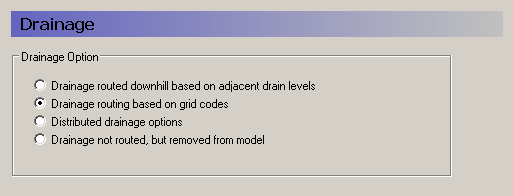
Drain Levels¶

The drainage recipient is calculated based on the drain levels in all the down gradient cells. That is, the location of the recipient cell is calculated as if the drain water was flowing downhill (based on the drain levels). This is the most common method of specifying drainage routing and the default setting.

Drain Codes¶

The drainage recipient is specified by the user based on a distribution map of integer code values.

Distributed option¶

With this option there are several different drainage possibilities, including a combination of Codes and Levels. The Distributed option can also be used to define a specific river model H-point or sewer manhole as a recipient.

Removed¶

The fourth option is simply a head dependent boundary that removes the drainage water from the model. This method does not involve routing and is exactly the same as the MODFLOW Drain boundary.

5. Groundwater wells¶

Groundwater wells can be included in your SZ simulation. The groundwater well locations, filter depth, pumping rates etc. are stored in a .wel file that is edited using the Well editor.

6. Linear reservoir groundwater method¶

In the linear reservoir method, the entire catchment is subdivided into a number of sub-catchments and within each subcatchment the saturated zone is represented by a series of interdependent, shallow interflow reservoirs, plus a number of separate, deep groundwater reservoirs that contribute to stream baseflow.

The lateral flows to the river (i.e. interflow and baseflow) are by default routed to the river links that neighbour the model cells in the lowest topographical zone in each subcatchment.

Interflow will be added as lateral flow to river links located in the lowest interflow storage in each catchment. Similarly, baseflow is added to river links located within the baseflow storage area.

Three Integer Grid Code maps are required for setting up the framework for the reservoirs,

a map with the division of the model area into sub-catchments,
a map of Interflow Reservoirs, and
a map of Baseflow Reservoirs.

The division of the model area into sub-catchments can be made arbitrarily. However, the Interflow Reservoirs must be numbered in a more restricted manner. Within each subcatchment, all water flows from the reservoir with the highest grid code number to the reservoir with the next lower grid code number, until the reservoir with the lowest grid code number within the subcatchment is reached. The reservoir with the lowest grid code number will then drain to the river links located in the reservoir.

For baseflow, the model area is subdivided into one or more Baseflow Reservoirs, which are not interconnected. However, each Baseflow Reservoir is further subdivided into two parallel reservoirs. The parallel reservoirs can be used to differentiate between fast and slow components of baseflow discharge and storage.

For more detailed information, see the section Linear Reservoir Method.