Saturated Zone
In MIKE SHE, the saturated zone is only one component of an integrated groundwater/surface water model. The saturated zone interacts with all of the other components - overland flow, unsaturated flow, channel flow, and evapotranspiration.
By comparison, MODFLOW only simulates the saturated flow. All of the other components are either ignored (e.g. overland flow) or are simple boundary conditions for the saturated zone (e.g. evapotranspiration).
On the other hand, there are very few differences between the MIKE SHE Finite Difference method and MODFLOW. The differences that are present are limited to differences in the discretisation and to some differences in the way some of the boundary conditions are defined.
Main saturated zone Dialog
The top dialog for the saturated zone section is slightly different depending on whether or not the Linear Reservoir Method or the 3D Finite Difference Method is chosen.
1. Linear Reservoir Method

Setting up a saturated groundwater model using the Linear Reservoir Method involves defining the Interflow and Baseflow Reservoirs, as well as their respective properties.
Pumping wells
By default, wells are not included, but in most applications pumping wells play a major role in the hydrology of the area. If wells are included in the model, then this must be checked and a new item in the data tree appears where the well database can be defined. Pumping wells extract water only from the baseflow reservoirs.
Related Items:
2. 3D Finite Difference Method
Setting up a saturated zone hydraulic model based on the 3D Finite Difference Method involves defining the:
- the geological model,
- the vertical numerical discretisation,
- the initial conditions, and
- the boundary conditions.
In the MIKE SHE GUI, the geological model and the vertical discretisation are essentially independent, while the initial conditions are defined as a property of the numerical layer. Similarly, subsurface boundary conditions are defined based on the numerical layers, while surface boundary conditions such as wells, drains and rivers are defined independently of the subsurface numerical layers.
The use of grid independent geology and boundary conditions provides a great deal of flexibility in the development of the saturated zone model, thus the same geological model and many of the boundary conditions can be reused for different model discretisation and different model areas.
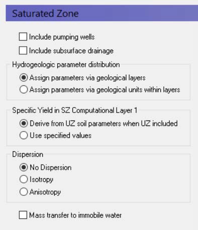
Include Pumping wells
By default, wells are not included, but in most applications pumping wells play a major role in the hydrology of the area. If wells are included in the model, then this must be checked and a new item in the data tree appears where the well database can be defined.
Include Subsurface drainage
Subsurface drainage is used to limit the amount of groundwater that reaches the ground surface and to route near surface groundwater to local streams and rivers. There are a number of drainage options for specifying surface drains in MIKE SHE, which are described in more detail in the section Drainage.
Hydrogeologic parameter distribution
The first option allows you to specify the hydrologic parameters of the geologic layers and lenses directly by means of .dfs2 grid files, point/line theme .shp files, or irregular xyz point values. The second option allows you to assign the hydrologic parameters to the geologic layers by means of zones with uniform properties, whereby the zones are defined by integer grid codes.
Specific Yield in SZ Computational Layer 1
By default, the specific yield in the top SZ layer is calculated from the specified UZ field capacity and saturated water content in the UZ layer that contains the initial water table. This is done to ensure the consistency between the SZ specific yield and the UZ properties. If these are inconsistent, then you may have a situation where the change in water table elevation in the UZ and the SZ models will be different.
You must specify a Specific Yield value for every SZ layer including the top SZ layer. However, when a UZ model is included in MIKE SHE, by default this value is not used. The Use specified values option allows you to over-ride the default. This may be a useful option to invoke if, for example, you are using Autocalibration. In this case, you can define and optimize the Specific Yield directly.
Dispersion
If your simulation includes water quality modelling in the saturated zone, then you must also define the type of dispersion you want to simulate. Dispersion is the physical process that causes solutes to spread longitudinally, vertically and horizontally as they move through the soil. The dispersion essentially represents the natural, microscopic variations in pore geometry that cause small scale variations in flow velocity.
No dispersion - Dispersion is ignored and no dispersivities need to be specified.
Isotropic - The transverse horizontal and transverse vertical dispersivities are assumed to be the same. Only two dispersivities need to be specified - the longitudinal and the transverse dispersivities.
Anisotropic - The horizontal and vertical transverse dispersivities are different, which requires the specification of five different dispersivities.
Mass Transfer to Immobile Water
If many cases, immobile water trapped in the bulk soil matrix is both a source and sink of solutes. In other words, as solutes move in the bulk water media, some of the solutes will diffuse into water trapped in the pores of the soil grains.
Furthermore, solutes in fractured media will be transported by diffusion in and out of the soil matrix. The porosity of the soil matrix is often at least ten times less than the fractures. The diffusion of solutes into the soil matrix will retard the initial breakthrough of the solute and the matrix will act as a long-term sink as the solute slowly diffuses out of the matrix long after the main solute plume has passed by.
If you turn on this option, then four additional data items may be required, namely
- the Secondary Porosity will be added as a geologic property,
- a Dual Porosity transfer coefficient per species will be required for each Water Quality layer,
- a Macropore/Secondary Half Life coefficient will be required for each species to calculate the solute decay in the matrix, and
- an initial concentration in the matrix for each species.
Note
There is no separate sorption process for the immobile water.
Related Items:
3. Interflow Reservoirs
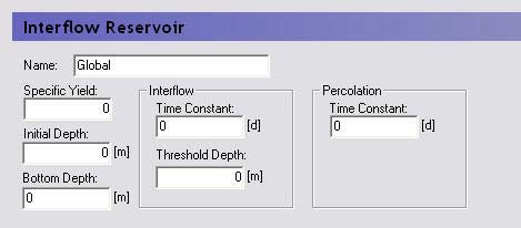
The interflow reservoirs are used to route near-surface groundwater to local streams. In the Linear Reservoir Method, each reservoir is assumed to be like a bathtub, with an inflow from infiltration and the upstream reservoir, as well as an outflow flowing into the next downstream reservoir and down into the baseflow reservoir beneath. Each linear reservoir flows only into the next downstream interflow reservoir, or into a stream if it is the lowest reservoir.
Note
Polygon shape files are currently not allowed for defining interflow reservoirs. The flow reference between interflow reservoirs depends precisely on the integer code numbers assigned to the reservoirs. Within a subcatchment, the interflow reservoir with the higher number always flows into the reservoir with the next lowest number.
Each Interflow reservoir requires a value for:
Specific Yield - to account for the fact that the reservoir contains a porous media and is not an actual bathtub.
Initial depth - the initial depth of water in the reservoir, measured from the ground surface.
Bottom depth - the depth below the ground surface of the bottom of the reservoir. If the water level drops to the bottom of the reservoir, percolation stops.
Interflow time constant - a calibration parameter that represents the time it takes for water to flow through the reservoir to the next reservoir.
Percolation time constant - a calibration parameter that represents the time it takes for water to seep down into the baseflow reservoir.
Interflow threshold depth - the depth below the ground surface when interflow stops. If interflow stops, percolation will continue until the reservoir is empty (i.e. the water level reaches the bottom depth). The threshold depth must be less than or equal to the depth to the bottom of the reservoir.
Related Items:
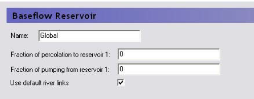
4. Baseflow Reservoirs
In the Linear Reservoir Method in MIKE SHE, each baseflow reservoir is divided into two parallel baseflow reservoirs. The two parallel baseflow reservoirs each receive a fraction of the percolation water from the interflow reservoirs as their only source of inflow. Each baseflow reservoir can discharge to pumping wells, to the unsaturated zone adjacent to streams and rivers (i.e. the zone beneath the lowest interflow reservoir), as well as directly to the river network.
In the primary baseflow reservoir map view, you can define the number of baseflow reservoirs in your system. You can define any number of baseflow reservoirs, but typically, there are only one or two.
For each baseflow reservoir pair, there are three items to define:
Fraction of percolation to reservoir 1 - this is used to divide the percolation between each of the two parallel baseflow reservoirs.
Fraction of pumping from reservoir 1 - this is used to divide the pumping (if it exists) between each of the two parallel baseflow reservoirs.
Use default river links - in most cases you will link the simplified overland flow and the groundwater interflow to all of the river links found in the lowest interflow reservoir in each subcatchment. However, in some cases you may want to link the flow to particular river links. For example, if your river network does not extend into the subcatchment, you can specify that the interflow discharges to a particular node or set of nodes in a nearby river network.
If you uncheck this checkbox, a River Links sub-item will appear where you can specify the river branch and chainage to link the subcatchment to.
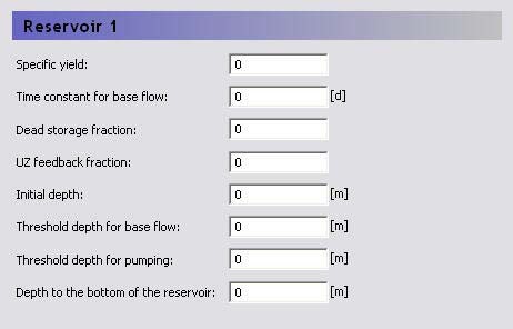
In the sub-Dialog for each of the parallel baseflow reservoirs, you must define the following:
Specific Yield - to account for the fact that the reservoir contains a porous media and is not an actual bathtub.
Time constant for base flow - a calibration parameter that represents the time it takes for water to flow through the reservoir.
Dead storage fraction - the fraction of the received percolation that is not added to the reservoir volume but is removed from the available storage in the reservoir.
UZ feedback fraction - the fraction of base flow to the river that is available to replenish the water deficit in the unsaturated zone adjacent to the river (i.e. the lowest interflow reservoir in the subcatchment).
Initial depth - the initial depth to the water in the reservoir measured from the ground surface.
Threshold depth for base flow - the depth below the ground surface when base flow stops. The threshold depth must be less than or equal to the depth to the bottom of the reservoir.
Threshold depth for pumping -the depth below the ground surface when pumping is shut off. The threshold depth must be less than or equal to the depth to the bottom of the reservoir.
Depth of the bottom of the reservoir - the depth below the ground surface of the bottom of the reservoir.
Related Items:
5. Geological Units
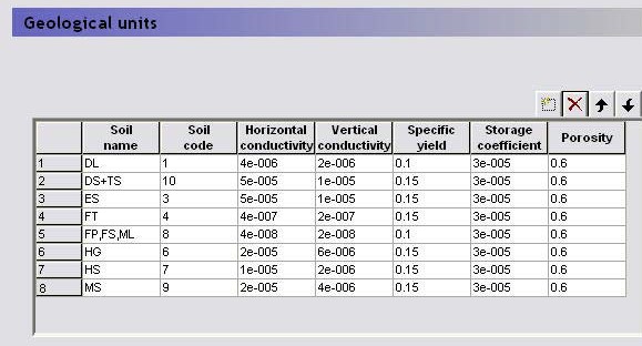
If you specify your geologic conceptual model via geological units, you can add each of your geologic units and its associated hydrogeologic properties to the table. Then, instead of specifying the hydrogeologic properties for each geological layer, you only need to specify the distribution of the units within the geologic layer or lense.
Related Items:
- Horizontal Hydraulic Conductivity
- Vertical Hydraulic Conductivity
- Specific Yield
- Specific Storage
- Porosity
- Dispersion Coefficients LHH, THH, TVH, LVV, THV
6. Geological Layers
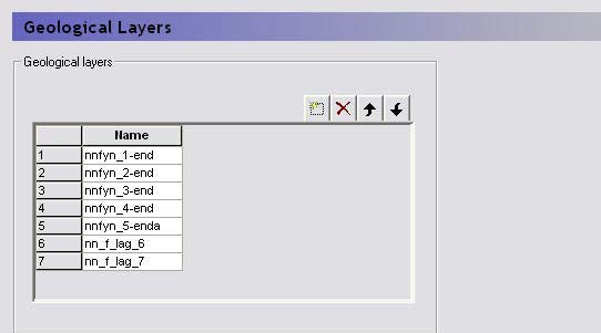
For each geologic layer, you must specify the hydrogeologic parameters of the layer including:
- Lower Level,
- Horizontal Hydraulic Conductivity,
- Vertical Hydraulic Conductivity,
- Specific Yield
- Specific Storage,
If you define your hydrogeology by , then most of the physical properties will be defined as properties of the Geological Unit and there will be an additional item, the Geological Unit Distribution, in the data tree.
Related Items:
7. Geological Lenses
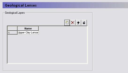
For each geologic layer, you must specify the hydrogeologic parameters of the layer including:
- Lower Level,
- Upper Level,
- Horizontal Extent,
- Horizontal Hydraulic Conductivity,
- Vertical Hydraulic Conductivity,
- Specific Yield,
- Specific Storage,
If you define your hydrogeology by , then most of the physical properties will be defined as properties of the Geological Unit and there will be an additional item, the Geological Unit Distribution, in the data tree.
Related Items:
8. Geological Unit Distribution
| Geological Unit Distribution | |
|---|---|
| Conditions | If geology defined by Geologic Units |
| Dialog Type | Integer Grid Codes |
| EUM Data Units | Grid Code |
| Valid Values | each value must be in the Geological Units table |
The Geological Unit Distribution references the geological units defined in the table. Each Integer Code must refer to one of the geological units in the table.
Related Items:
9. Horizontal Hydraulic Conductivity
| Horizontal Hydraulic Conductivity | |
|---|---|
| Dialog Type | Stationary Real Data |
| EUM Data Units | HydrConductivity |
The hydraulic conductivity is a function of the soil texture and is related to the ease with which water can flow through the soil. Loose, coarse uniform soils have a higher conductivity than compacted soils with a range of particle sizes. Thus, a loose, uniform coarse sand can have a horizontal hydraulic conductivity as high as 0.001 m/s. Whereas, a tight, compacted clay can have a have a horizontal hydraulic conductivity as low as 1x10⁻⁸ m/s - which is 5 orders of magnitude.
The horizontal hydraulic conductivity is typically 5 to 10 times higher than the vertical hydraulic conductivity.
MIKE SHE assumes that the horizontal conductivity is isotropic in the x and y directions.
Related Items:
10. Vertical Hydraulic Conductivity
| Vertical Hydraulic Conductivity | |
|---|---|
| Dialog Type | Stationary Real Data |
| EUM Data Units | HydrConductivity |
The hydraulic conductivity is a function of the soil texture and is related to the ease with which water can flow through the soil. Loose, coarse uniform soils have a higher conductivity than compacted soils with a range of particle sizes. Thus, a loose, uniform coarse sand can have a horizontal hydraulic conductivity as high as 0.001 m/s. Whereas, a tight, compacted clay can have a have a horizontal hydraulic conductivity as low as 1x10⁻⁸ m/s - which is 5 orders of magnitude.
The vertical hydraulic conductivity is typically 5 to 10 times lower than the horizontal hydraulic conductivity.
Related Items:
11. Specific Yield
| Specific Yield | |
|---|---|
| Dialog Type | Stationary Real Data |
| EUM Data Units | Specific Yield |
In an unconfined aquifer, the Specific Yield is defined as the volume of water released per unit surface area of aquifer per unit decline in head. The specific yield is much higher than the Specific Storage because the water that is released is primarily from the dewatering of the pores at the water table. This results in a unit of L3/L2/L, which is dimensionless. The Specific Yield is only used in transient simulations but must always be input. Furthermore, the specific yield is only used in the cells that contain the water table. In the cells below the water table, the Specific Storage is used.
Specific Yield of upper SZ layer
The specified value for specific yield is not used for the specific yield of the upper most SZ layer if UZ is included in the simulation.
By definition, the specific yield is the amount of water release from storage when the water table falls. The field capacity of a soil is the remaining water content after a period of free drainage. Thus, specific yield is equal to the saturated water content minus the field capacity.
To avoid water balance errors at the interface between the SZ and UZ models, the specific yield of the top SZ layer is set equal to the he saturated water content minus the field capacity. The value is determined once at the beginning of the simulation. The water content parameters are taken from the UZ layer in which the initial SZ water table is located.
Related Items:
12. Specific Storage
| Specific Storage | |
|---|---|
| Dialog Type | Stationary Real Data |
| EUM Data Units | Elastic Storage |
In a confined aquifer, the specific storage is defined as the volume of water released per volume of aquifer per unit decline in head. This is slightly different than the specific yield because the water released from storage comes primarily from the expansion of the water and aquifer compression due to the reduction in water pressure (increase in effective stress). Thus, the water released from storage is released from the entire column of water in the aquifer, not just at the phreatic surface. This results in a unit of L3/L3/L, or 1/L.
The Specific Storage Coefficient is only used in transient simulations but must always be input. Furthermore, the specific storage coefficient is only used in the cells below the water table. In the cells containing the water table, the Specific Yield is used.
13. Porosity
| Porosity | |
|---|---|
| Conditions | if the Include Advection Dispersion (AD)Water Quality option selected in the SimulationSpecification Dialog |
| Dialog Type | Stationary Real Data |
| EUM Data Units | Porosity |
In a porous media, most of the volume is taken up by soil particles and the actual area available for flow is much less than the nominal area. This distinction is important when calculating flow velocities for solute transport. The porosity is the cross-sectional area available for flow divided by the nominal cross-sectional area. This is often referred to as the effective porosity, since it discounts the dead end pore spaces that are not available for flow. In the absences of dead end pores, the porosity is equal to the specific yield.
The Porosity must be greater than 0 and less than 1. For unconsolidated porous media, the porosity is usually from 0.15 to 0.3 depending on the grain size distribution (the more uniform the higher the effective porosity). For fractured media the porosity is usually much lower, in the from 0.01 to 0.05.
Related Items:
14. Secondary Porosity
| Secondary Porosity | |
|---|---|
| Conditions | if the Include Advection Dispersion (AD) Water Quality option selected in the Simulation Specification dialog AND if the Mass Transfer to Immobile Water option selected in the Saturated Zone dialog |
| Dialog Type | Stationary Real Data |
| EUM Data Units | Porosity |
Solutes travelling in a fractured media will be transported by diffusion into and out of the soil matrix of the surrounding media. The velocity in fractured media due to the lower effective porosity will cause very fast break-through down gradient. However, the solute mass that diffuses into the surrounding media will act like a long-term solute source after the main plume has passed, as the solute diffuses back into the fractures.
The matrix source/sink process can be included in MIKE SHE by activating the Mass Transfer to Immobile Water option in the Saturated Zone dialog.
Matrix porosity must be between 0 and 1. Matrix porosities are generally very difficult to measure and are usually calibrated against breakthrough curves to estimate a realistic value. Furthermore, the value needs to be the "effective" matrix porosity - that is, the matrix porosity that is "actively" involved in solute diffusion. This can be significantly lower than the matrix porosity measured by core analysis. For a limestone aquifer the matrix porosity has been calibrated to be as small as 4 per cent (core samples indicated 20 to 35%) whereas for a clay till sample it was calibrated to be 20 to 30% - a little less than the total matrix porosity.
Related Items:
- Dual Porosity transfer coefficient
- Solute Transport in the Saturated Zone
- Transport in Fractured Media
15. Bulk Density
| Bulk Density | |
|---|---|
| Conditions | if the Include Advection Dispersion (AD) Water Quality option selected in the Simulation Specification Dialog AND the SZ solute transport option is turned on AND at least one sorption process is active |
| Dialog Type | Stationary Real Data |
| EUM Data Units | Density |
The bulk density is the average density of the in-place soil material, including void space. In other words, if you were to remove one cubic meter of soil, how much would it weigh? A typical bulk density is about 1700 kg/m3, but representative local values are usually available.
The bulk density is used in the calculation of sorption of solutes, so you need to specify a bulk density whenever any sorption processes are active in SZ.
Related Items:
16. Dispersion Coefficients LHH, THH, TVH, LVV, THV
| AUG | |
|---|---|
| Dialog Type | Stationary Real Data |
| EUM Data Units | Dispersion Coefficient |
If dispersion is included, then the two different dispersion options differ in the number of dispersion parameters required. If you assume isotropic conditions you need to specify the longitudinal dispersivity, \(\beta_L\), and the transversal dispersivity, \(\beta_T\) . If you assume anisotropic conditions, you need to specify five dispersivities.
The magnitude of the dispersivity coefficient depends on the degree of heterogeneity in your geology and the degree to which these heterogeneities have been described in the model. The more heterogeneous your geology is, the larger the dispersivities should be. On the other hand, the more detailed you have described the heterogeneities with your model geometry, the smaller dispersivities should be.
Further, the magnitude of the dispersivities depends on the size of the model and on the model grid size. The larger the model, the larger the dispersivities should be. Whereas the larger the grid size, the smaller the dispersivities should be due to numerical dispersion.
Thus, it is difficult to give a rule of thumb for the values of dispersivity. Recent field experiments on solute transport, though, indicate that the longitudinal dispersivity should be in the range of 1% or less of the travel distance, the transverse-horizontal dispersivity should be at least 50 times less than this and the transverse-vertical dispersivity should be 2 or more times less than the transverse-horizontal.
Related Items:
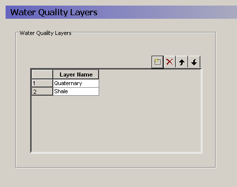
17. Water Quality Layers
| Water Quality Layers | |
|---|---|
| Conditions | if the Include Advection Dispersion (AD) Water Quality option selected in the Simulation Specification Dialog AND the SZ solute transport option is turned on AND at least one sorption or decay process is active |
The water quality layers present a conceptual layer system like the geologic layers that applies to chemistry parameters. In some cases, the water quality layers will mimic the geologic layers, but in other case they will not. For example, redox potential will not generally follow the geologic layers and water quality parameters related reaction processes will be quite different in oxidizing and reducing environments. Likewise, you may have several geologic layers in the upper quaternary deposits that affect the flow hydraulics, but the water chemistry can be divided into a quaternary sand and silt zone overlain on an iron rich shale layer.
Unfortunately, the different water quality parameters may not all require identical water quality layers. However, in the current version, only one set of water quality layers is available. If two or more parameters require different distributions, then you will have to divide the overlapping layers into separate units.
When you add a Water Quality Layer to the table, an item is added to the data tree containing all of the relevant data for the Water Quality Decay Processes and Water Quality Sorption processes that are active. The location of the WQ Layer is specified by a Lower Level.
Related Items:
- Solute Transport in the Saturated Zone
- Water Quality Decay Processes
- Water Quality Sorption processes
- Lower Level
18. Dual Porosity transfer coefficient
| Mass transfer coefficient to immobile water | |
|---|---|
| Dialog Type | Stationary Real Data |
| EUM Data Units |
Solutes travelling in a fractured media will be transported by diffusion into and out of the soil matrix of the surrounding media. The velocity in fractured media due to the lower effective porosity will cause very fast break-through down gradient. However, the solute mass that diffuses into the surrounding media will act like a long-term solute source after the main plume has passed, as the solute diffuses back into the fractures.
The matrix source/sink process can be included in MIKE SHE by activating the Mass Transfer to Immobile Water option in the Saturated Zone dialog.
The mass transfer coefficient represents the rate at which mass is transferred between the fractures and the matrix. It depends on the geology and chemistry. It is defined per species.
Related Items:
19. Computational Layers
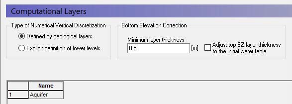
The vertical discretisation in the saturated zone can be defined in two ways:
- by the geological layers, in which case there will be one calculation node in each geological layer,
- by explicitly defining the lower level of each calculation layer.
Vertical discretisation
Defined by the geological layers - Groundwater flow in a multi-layer aquifer can be described by a model in which the computational layers follow the interpreted geological layers. Each layer is characterised only by its base level specified either by a constant level or by a distributed file. The number of numerical layers will be identical with the number of geologic layers.
Explicit definition of lower levels - If you define the vertical discretisation explicitly each computational layer is defined by its lower elevation.
Bottom elevation correction
There are two corrections that may be made to the layer elevations.
Minimum layer thickness – The minimum thickness of the calculation layers must be specified to adjust the geological model or the specified levels to prevent layers with zero thickness or very thin layers. Otherwise, very thin layers may cause numerical difficulties. The default value is 0.5, which is usually sufficient. This means that if the two geological layers or specified layer elevations approach one another then the bottom layer will be pushed down to maintain the minimum layer thickness. When explicitly defining computational layers or when the model contains any geological lenses: Any layers entirely pushed below the specified bottom of the model will be assigned a hydraulic conductivity (both horizontal and vertical) of 1e-20 m/s. If a layer is just partially pushed below the bottom of the model the conductivities will be averaged between the specified values and 1e-20 m/s.
Adjust top SZ layer thickness to the initial water table - In principle, the UZ calculates vertical infiltration in the unsaturated zone and the SZ calculates 3D saturated flow below the water table. However, the UZ and SZ layer elevations are defined independently of one another. In MIKE SHE, the UZ flow is only calculated to the water table, or to the bottom of top SZ layer. Any UZ cells below this are ignored and outflow from the UZ model is added to the top layer of the SZ model. This option allows you to more easily keep the UZ and SZ models consistent based on the depth of the initial SZ water table.
The adjustment is made during preprocessing and uses the Initial Potential Head of the top computational layer (limited upwards by the topography). Heads from a hot start file are not considered - the layer geometry is fixed before the hot start data is read. If you hot start and want the top layer to capture the hot start water table, specify the Initial Potential Head of the top layer accordingly, for example from the "elevation of top phreatic surface" result item of the previous run: extract the time step at the hot start date into a single-time-step dfs2 (the item type, Elevation, matches directly - and note that only the first time step of a dfs2 is read here). In a hot-started run the actual starting heads still come from the hot start file, so the Initial Potential Head then only affects the layer geometry.
Related Items:
- Coupling the Unsaturated Zone to the Saturated Zone
- Definition of vertical UZ numerical grid
- Saturated Flow - Technical Reference
20. Initial Potential Head
| Initial Potential Head | |
|---|---|
| Dialog Type | Stationary Real Data |
| EUM Data Units | Elevation |
The Initial Potential Head is the starting head for transient simulations and the initial guess for steady-state simulations. The choice of initial head for steady state simulations may affect the rate of numerical convergence depending on the solver used.
Related Items:
21. Initial Soil Temperature
The initial soil temperature is required if temperature dependent decay is specified. The current soil temperature is calculated at every time step based on an empirical formula using the air temperature.
Related Items:
22. Outer boundary conditions
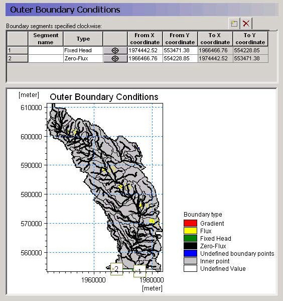
The outer boundary conditions are defined as line segments between two boundary points. The boundary points are, in principle, independent of the model domain because they do not need to lie on the model boundary.
Rather they are projected onto the nearest model boundary cell. Thus, the model boundary can be modified slightly without having to modify the boundary locations. However, if the model boundary is moved significantly or if the boundary is convoluted then the calculated ‘nearest’ node might not be the one expected.
Specifying a boundary condition
To specify an outer boundary segment,
- add a new line to the outer boundary points table,
- click on the target icon,
- click on one end of your boundary segment,
- add a second line to the outer boundary points table,
- click on the new target icon,
- click on the other end of your boundary segment,
- Change the name of the top line of the points table,
- Select the appropriate boundary condition for the boundary segment.
Available boundary conditions
Fixed Head - This boundary prescribes a head in the boundary cell. The head can be fixed at a prescribed value, fixed at the initial value from the initial conditions, or assigned to a .dfs0 time series file. If a time series input is used, then the actual value used in the model at the current time step is linearly interpolated from the available values. The last option is a time varying dfs2 file, which is typically extracted from a regional results file. This can be done using the MIKE Zero Toolbox Extraction tool: 2D Grid from 3D files. MIKE SHE then interpolates in both time and space from the .dfs2 file to the local head boundary at each local time step.
Zero flux - This is a no-flow boundary, which is the default.
Flux - This boundary prescribes a flux across the outer boundary of the model. When the spatial distribution is set to "global", the given value will designate the total inflow along the entire boundary stretch, which may contain several cells. A time varying flux can be specified as a mean step-accumulated discharge (e.g. m³/s) or as a step-accumulated volume (e.g. m³). A positive value implies an inflow to the model cells.
When the spatial distribution is set to "distributed" the boundary inflow can be specified for each cell in the boundary stretch separately. Also, the inflow along x- and y-axis can be specified individually. As before, a positive value implies an inflow to the model cells.
Gradient - This boundary describes a constant or time varying gradient between the node on the outer boundary and the first internal node. A time varying gradient can be specified as an instantaneous dimensionless or percent value. A positive gradient implies a flux into the model.
Notes
- The head is calculated in a No Flow outer boundary cells, whereas the head is specified in the Fixed Head outer boundary cells, but in both cases all properties must be assigned to all outer boundary cells.
- An internal model cell in contact with multiple boundary cells will not receive multiple quantities of water.
- Additional detailed information can be found under Boundary Conditions in the Saturated Flow - Technical Reference.
- An error will be generated if the flux/gradient input cell:
- has zero thickness,
- has a horizontal hydraulic conductivity of zero,
- is an inactive internal boundary cell, or
- is a fixed head internal boundary cell. - A warning will be issued if the flux/gradient boundary:
- is a head-controlled flux (GHB) internal boundary cell, or
- is a fixed head drain internal boundary cell.
Related Items:
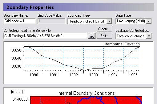
23. Internal Boundary Conditions
| Internal Boundary Conditions | |
|---|---|
| Dialog Type | Integer Grid Codes with sub-Dialog data |
| EUM Data Units | Grid Code |
The map Dialog for the internal boundary conditions allows you to specify the locations of the various boundary conditions. Any Integer Code value is permissible, and a separate item will be added to the data tree below this level with one item for each unique integer code in the domain.
Only one integer code is allowed per cell, which means that no cell can have more than one boundary condition.
If you use a polygon .shp file, each unique polygon will have a separate entry in the data tree.
Available boundary conditions
The following boundary conditions can be defined for each integer code:
Fixed Head For a fixed head boundary, you specify the head in the cell. The model will not calculate the head in the cell. Care should be taken when specifying fixed head boundary conditions, as the cell becomes an infinite source or sink of water. The fixed head can be a prescribed value, fixed at the initial value from the initial conditions, assigned to a .dfs0 time series file, or assigned to a time varying dfs2 file. The last option is typically from a results file. It could be from a regional results file, which can be extracted using the MIKE Zero Toolbox Extraction tool: 2D Grid from 3D files. Or it could be from a previous run of the same model.
Fixed Head Drain - For a fixed head drain boundary, you specify a reference head. If the cell water level is above the reference level, then the boundary acts like a normal fixed head boundary condition. If the head in the cell falls below the reference level, then the boundary condition is turned off. That is, if the simulated head drops below the head reference level the flux is set to zero. Thus, the fixed head drain allows only water extraction.
The reference head can be a prescribed value, fixed at the initial value from the initial conditions, assigned to a .dfs0 time series file, or assigned to a time varying dfs2 file. The last option is typically from a results file. It could be from a regional results file, which can be extracted using the MIKE Zero Toolbox Extraction tool: 2D Grid from 3D files. Or it could be from a previous run of the same model.
Note
This boundary condition was previously called the Head controlled abstraction boundary condition in early versions of MIKE SHE.
Head Controlled Flux (GHB) - The head controlled flux, or General Internal Head Boundary is similar to the fixed head. However, a flow resistance is incorporated via a user specified leakage coefficient.
The head can be a prescribed value, assigned to a .dfs0 time series file, or assigned to a time varying dfs2 file. The last option is typically from a results file. It could be from a regional results file, which can be extracted using the MIKE Zero Toolbox Extraction tool: 2D Grid from 3D files. Or it could be from a previous run of the same model.
If the GHB is selected, an extra item is added to the data tree below the boundary condition for the leakage coefficient. The leakage coefficient can be specified as either a simple leakage coefficient [1/time] or as a total conductance [length2/time].
Note
This boundary condition was previously called the General Internal Head Boundary condition in early versions of MIKE SHE
Inactive Cells - This boundary condition is used to make interior cells of the model inactive. It works by assigning a hydraulic conductivity of zero to the cells if the simulation is transient, or a value of 10-15 if the simulation is steady state. Note, though, that this method means that in the pre-processed data, you will see the inactive cells show up in the maps of hydraulic conductivity rather than in the maps of boundary conditions. Also note that since the inactive cells are actually active cells with zero conductivity, the results will also include head values in these points.
Related Items:
24. Initial (secondary) concentration
| Internal Boundary Conditions | |
|---|---|
| Conditions | if the Include Advection Dispersion (AD) Water Quality option selected in the Simulation Specification dialog |
| Dialog Type | Stationary Real Data |
| EUM Data Units | Concentration |
There is an initial concentration item for each computational layer. Under each initial concentration item, there is one sub-item for each active species.
The initial concentration is used by the MIKE SHE Water AD engine as the starting concentration for the Water quality simulation.
If you have specified Mass Transfer to Immobile Water option selected in the Saturated Zone dialog, then you will also have to specify an initial concentration in the immobile water located in the secondary (matrix) porosity.
Related Items:
25. Initial number of particles per cell
| Initial number of particles per cell | |
|---|---|
| Conditions | if the Include Advection Dispersion (AD) Water Quality option selected in the Simulation Specification dialog and the Random walk particle tracking sub-option is specified and the initial particle density is specified as a number of particles. |
| Dialog Type | Stationary Real Data |
| EUM Data Units | Integer |
There is an initial number of particles item for each computational layer. The initial number of particles is used by the MIKE SHE Random Walk particle tracking engine as the starting concentration.
Related Items:
26. PT Registration Codes/Lenses
| PT Registration Codes/Lenses | |
|---|---|
| Conditions | if the Include Advection Dispersion (AD) Water Quality option selected in the Simulation Specification dialog and the Random walk particle tracking sub-option is specified and PT Registration codes are defined by layer or lense |
| Dialog Type | Stationary Real Data |
| EUM Data Units | Integer |
When you run the random walk particle tracking option, registration areas can be defined. All particles passing through a registration area will be tagged.
This allows you to create a point shape file that contains the starting location of all particles that passed through the registration area.
Registration codes by layer
If you specify the registration codes by layer, then you can specify a dfs2 integer grid code array for each numerical layer. Each unique integer codes will be used as a registration zone.
Registration codes by lenses
If you specify the registration zones by lenses, then you have to specify an Horizontal Extent, as well as an Upper Level and a Lower Level for the lense. This is a more flexible way to define the registration zone but is significantly slower because every particle has to be checked against the extent and the top and bottom elevations.
Related Items:
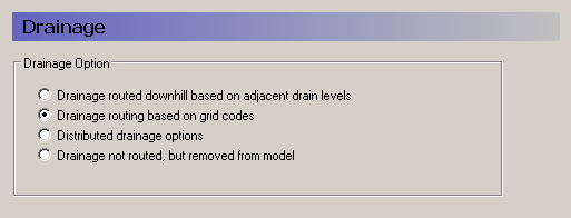
27. Drainage
Saturated zone drainage is a special boundary condition in MIKE SHE used to define natural and artificial drainage systems that cannot be defined in MIKE 1D. It can also be used to simulate simple overland flow in a lumped conceptual approach. Saturated zone drainage is applied to the layer of the Saturated Zone model containing the drain level. Water that is removed from the saturated zone by drains is routed to local surface water bodies.
Drain flow is simulated using an empirical formula. Each cell requires a drain level and a time constant (leakage factor). Both drain levels and time constants can be spatially defined. A typical drainage level is 1m below the ground surface and a typical time constant is between 1e-6 and 1e-7 1/s.
MIKE SHE also requires a reference system for linking the drainage to a recipient node or cell. The recipient can be a river node, another SZ grid cell, or a model boundary. Whenever drain flow is produced during a simulation, the computed drain flow is routed to the recipient point using a linear reservoir routing technique.
Drainage routed downhill based on adjacent drain levels
This option was originally the only option in MIKE SHE. The reference system is created automatically by the pre-processor using the slope of the drains calculated from the drainage levels in each cell.
Thus, the pre-processer calculates the drainage source-recipient reference system by
- looking at each cell in turn and then
- look for the neighbouring cell with the lowest drain level.
- If this cell is an outer boundary cell or contains a river link, the search stops.
If the cell does not contain a boundary or river link, then the next search is repeated until either a local minimum is found, or a boundary cell or river link is located.
The result of the above search for each cell is used to build the source-recipient reference system.
If local depressions in the drainage levels exist, the SZ nodes in these depressions may become the recipients for a number of drain flow producing nodes. This often results in the creation of a small lake at such local depressions. If overland flow is simulated, then the drainage water will become part of the local overland flow system.
Note
Be aware that the drainage is routed to a destination. It does not physically flow downhill. The drain levels are only used to build the drainage source-recipient reference system. In other words, any drainage that is generated at a node, is immediately moved to the recipient node. The assumption here, is that the time step length is longer than the time it takes for the drainage to reach its destination.
Drainage routing based on grid codes
This method is often used when the topography is very flat, which can result in artificial depressions, or when the drainage system is very well defined, such as in agricultural applications.
In this method, the drainage levels and the time constants are defined as in the previous method and the amount of drainage is calculated based on the drain levels and the time constant.
If the drainage routing is specified by Drain Codes, a grid code map is required that is used to restrict the search area for the source-recipient reference system. In this case, the pre-processer calculates the reference system within each grid code zone, such that all drainage generated within one zone is routed to recipient nodes with the same drain code value.
When building the reference system, the pre-processor looks at each cell and then
- looks for the nearest cell with a river link with the same grid code value,
- if there are no cells with river links, then it looks for the nearest outer boundary cell with the same grid code,
- if there are no cells with outer boundary conditions, then it looks for the cell with the same grid code value that has the lowest drain level.
The result of the above search for each cell is used to build the source-recipient reference system.
The above search algorithm is valid for all positive Drain Code values. However, all cells where:
Drain Code = 0 - will not produce any drain flow and will not receive any drain flow, and
Drain Code < 0 (negative) - will not drain to river links but will start at Step 2 above and only drain to either an outer boundary or the lowest drain level.
Distributed drainage options
Choosing this method, adds the Option Distribution item to the data tree. With the Option Distribution, you can specify an integer grid code distribution that can be used to specify different drainage options in different areas of your model.
Code = 1 - In grid cells with a value of 1, the drainage reference system is calculated based on the Drain Levels.
Code =2 - In grid cells with a value of 2, the drainage reference system is calculated based the Drain Codes.
Code = 3 - Drainage in grid cells with a value of 3 is routed to a specified Branch and chainage. At the moment, this option requires the use of Extra Parameters and is described in SZ Drainage to Specified River H-points.
Code = 4 - Drainage in grid cells with a value of 4 is routed to a specified sewer manhole. This option is described in the section Working with Sewers - User Guide.
Drain flow not routed, by removed from model
The fourth option is simply a head dependent boundary that removes the drainage water from the model. This method does not involve routing and is exactly the same as the MODFLOW Drain boundary.
Related Items:
- Groundwater drainage
- Saturated Zone Drainage
- SZ Drainage to Specified River H-points
- Coupling of MIKE SHE and a MIKE 1D Sewer Model
28. Drain Level
| Drain Level | |
|---|---|
| Dialog Type | Stationary Real Data |
| EUM Data Units | Elevation |
If surface drainage is routed by drain levels, the drainage routing reference system is created automatically using the slope of the drains calculated from the drainage levels in each cell.
The drain levels are only used for two things:
- to calculate the drain cell-drain recipient relations, and
- to calculate the amount of drain flow produced in each node when the water table is above the drain level.
The drain level also determines from which SZ layer the drain water will be extracted.
Warning
If the drain level is set equal to the topography in a cell, then the drainage will be turned off in the cell. Drain levels above the topography are not allowed. In this case, the drain level will be automatically adjusted to just below the topography.
Related Items:
- Drainage
- Groundwater drainage
- Saturated Zone Drainage
- SZ Drainage to Specified River H-points
- Coupling of MIKE SHE and a MIKE 1D Sewer Model
29. Drain Time Constant
| Drain Time Constant | |
|---|---|
| Dialog Type | Stationary Real Data |
| EUM Data Units | Leakage Coefficient./Drain Time Constant |
Drainage flow is simulated using an empirical formula that requires a drainage level and a time constant (leakage factor) for each cell. Mathematically, the time constant is exactly the same as a leakage coefficient - it is simply a factor that is used to regulate how quickly the water can drain. A typical time constant is between 1e-6 and 1e-7 1/s.
Related Items:
- Drainage
- Groundwater drainage
- Saturated Zone Drainage
- SZ Drainage to Specified River H-points
- Coupling of MIKE SHE and a MIKE 1D Sewer Model
30. Drain Codes
| Drain Codes | |
|---|---|
| Dialog Type | Integer Grid Codes |
| EUM Data Units | Grid Code |
If the drainage routing is specified by Drain Codes, a grid code map is required that is used to link the drain flow producing cells to recipient grid cells. The drain levels are still used to calculate the amount of drain flow produced in each node, but the routing is based only on the code values in the drain code file.
The Drain Code can be any integer value, but the different values have the following special meanings:
Code = 0 - Grid cells with a Drain Code value of zero will not produce any drain flow and will not receive any drain flow.
Code > 0 - Grid cells with positive Drain Code values will drain to the nearest river, boundary or local depression in the drain level - in that priority - located next to a cell with the same Drain Code value. Thus, if a grid cell produces drainage,
- If there are one or more cells with the same drain code next to a river link, then the drain flow will be routed to the nearest of these cells.
- If there are no cells with the same Drain Code located next to a river link, then the drain flow will be routed to the nearest boundary cell with the same Drain Code value.
- If there are no boundary cells with the same Drain Code value, the drain flow will be routed to the cell with the lowest drain level that has the same Drain Code value (which may create a lake).
Code < 0 - Grid cells with negative Drain Code values will drain to either a boundary or a local depression, in that order. Thus, if a grid cell produces drainage,
- If there are no cells with the same Drain Code located next to a river link, then the drain flow will be routed to the nearest boundary cell 2ith the same Drain Code value.
- If there are no boundary cells with the same Drain Code value, the drain flow will be routed to the cell with the lowest drain level that has the same Drain Code value (which may create a lake).
Related Items:
- Drainage
- Groundwater drainage
- SZ Drainage to Specified River H-points
- Coupling of MIKE SHE and a MIKE 1D Sewer Model
31. Option Distribution
| Option Distribution | |
|---|---|
| Conditions | always when Surface Drainage active AND when the Distributed drainage option is used. |
| Dialog Type | Integer Grid Codes |
| EUM Data Units | Grid Code |
| Valid Values: | 1, 2, 3 and 4 only |
The drain type distribution is used to distinguish areas of the model where different drainage options are used.
Code = 1 - Drainage in grid cells with a value of 1 is routed downhill based on the value of the drain level specified in Drain Level data item.
Code =2 - Drainage in grid cells with a value of 2 is routed via Drain Codes as specified in the Drain Codes data item.
Code = 3 - Drainage in grid cells with a value of 3 is routed to a specified branch and chainage. At the moment, this option requires the use of Extra Parameters.
Code = 4 - Drainage in grid cells with a value of 4 is routed to a specified sewer manhole. At the moment, this options requires the use of Extra Parameters.
Related Items:
- Saturated Zone Drainage
- Extra Parameters
- SZ Drainage to Specified River H-points
- Coupling of MIKE SHE and a MIKE 1D Sewer Model
32. Pumping Wells
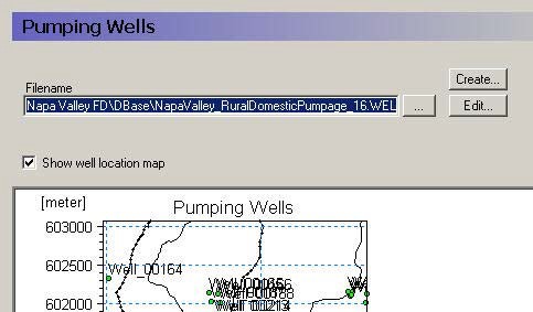
If pumping wells are active in the model domain, then you must specify the name of the well database to include in the model setup.
Edit The Edit button will open the current Well Database with the current maps and overlays open in the well editor.
You may get an error in when you open the Well Database if the model has not yet been pre-processed or if the model data has changed without re-preprocessing the model. This error happens because MIKE SHE is trying to reconcile and plot both the geologic layers (input data) and the numerical layers (preprocessed data) for each cell containing a pumping well.
Create The Create button will create a new Well Database file