3D Finite Difference Method

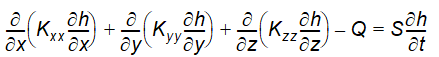
The governing flow equation for three-dimensional saturated flow in saturated porous media is:

Equation 33.01

where - Kxx,Kyy,Kzz the hydraulic conductivity along the x, y and z axes of the model, which are assumed to be parallel to the principle axes of hydraulic conductivity tensor - h is the hydraulic head - Q represents the source/sink terms - S is the storage coefficient.

Two special features of this apparently straightforward elliptic equation should be noted. First, the equations are non-linear when flow is unconfined and, second, the storage coefficient is not constant but switches between the specific storage coefficient for confined conditions and the specific yield for unconfined conditions.

1. The Pre-conditioned Conjugate Gradient (PCG) Solver

As an alternative to the SOR-solver, MIKE SHE’s groundwater component also includes the pre-conditioned conjugate gradient solver (Hill, 1990). The PCG solver includes both an inner iteration loop, where the head dependent boundaries are kept constant, and an outer iteration loop where the (non-linear) head dependent terms are updated. The PCG solver includes a number of additional solver options that are used to improve convergence of the solver. The default values will generally ensure good performance. For the majority of applications, there is no need to adjust the default solver settings. If, on the other hand, non-convergence or extremely slow convergence is encountered in the SZ component, then some adjustment of the solver settings may help.

The PCG solver in MIKE SHE, which is identical to the one used in MODFLOW (McDonald and Harbaugh, 1988), requires a slightly different formulation of the hydraulic terms when compared to the SOR solver.

a. Potential flow terms

The potential flow is calculated using Darcy's law

Equation 33.02

where - Dh is the piezometric head difference - C is the conductance.

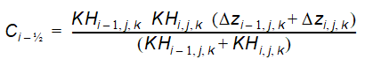
The horizontal conductance in Eq. (33.2) is derived from the harmonic mean of the horizontal conductivity and the geometric mean of the layer thickness. Thus, the horizontal conductance between node i and node i-1 will be

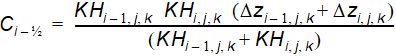
Equation 33.03

where - KH is the horizontal hydraulic conductivity of the cell - \(\Delta z\) is the saturated layer thickness of the cell

The vertical conductance between two cells is computed as a weighted serial connection of the hydraulic conductivity, calculated from the middle of layer k to the middle of the layer k+1. Thus,

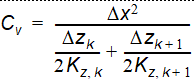
Equation 33.04

where - Dz is the layer thickness

Dewatering conditions

Consider the situation in Figure 33.1, where the cell below becomes dewatered.

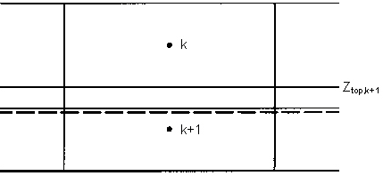
Figure 33.1 Dewatering conditions in a lower cell.

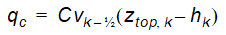
The actual flow between cell k and k+1 is

Equation 33.05

In the present solution scheme the flow will be computed as

Equation 33.06

Subtracting Eqs.(33.5) from (33.6) gives the correction term

Equation 33.07

which is added to the right-hand side of the finite difference equation using the last computed head.

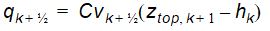
A correction must also be applied to the finite difference equation if the cell above becomes dewatered.

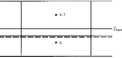
Figure 33.2 Dewatering conditions in the cell above

Thus, from Figure 33.2, the flow from cell k-1 to k is

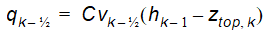
Equation 33.08

where, again the computed flow is

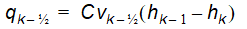
Equation 33.09

Subtracting Eqs. (33.8) from (33.9) gives the correction term

Equation 33.10

which is added to the right-hand side of the finite difference equation using the last computed head

b. Storage terms

The storage capacity is computed by

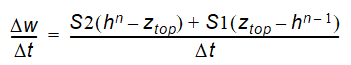
Equation 33.11

where - n is time step - S1 is the storage capacity at the start of the iteration at time step n, - S2 is the storage capacity at the last iteration.

For confined cells the storage capacity is given as

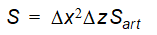
Equation 33.12

and for unconfined cells the storage capacity is given as

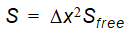
Equation 33.13

c. Maximum Residual Error

The maximum residual error is the largest allowable value of residual error during an iteration. The solution is obtained when the residual error during an iteration in any computational node is less than the specified tolerance.

The value of the maximum residual error should be selected according to aquifer properties and the dimensions of the model. In practice the maximum residual error value will always be a compromise between accuracy and computing time. It is recommended to check the water balance carefully at the end of the simulation, but it should be emphasized that large internal water balance errors between adjacent computational nodes may not be detected.

If large errors in the water balance are produced the maximum residual error should be reduced.

d. Gradual activation of SZ drainage

To prevent numerical oscillations the drainage constant may be adjusted between 0 and the actual drainage time constant defined in the input for SZ drainage. The option has been found to have a dampening effect when the groundwater table fluctuates around the drainage level between iterations (and does not entail reductions in the drain flow in the final solution).

e. Mean values of horizontal SZ-conductance:

To prevent potential oscillations of the numerical scheme when rapid changes between dry and wet conditions occur a mean conductance is applied by taking the conductance of the previous (outer) iteration into account.

f. Under relaxation

The PCG solver can optionally use an under-relaxation factor between 0.0 and 1.0 to improve convergence. In general a low value will lead to convergence, but at a slower convergence rate (i.e. with many SZ iterations). Higher values will increase the convergence rate, but at the risk of non-convergence.

Automatic (dynamic) estimation of under-relaxation factors

If the automatic estimation of the under-relaxation factor is allowed, the under-relaxation factor is calculated automatically as part of the outer iteration loop in the PCG solver. The algorithm determines the factors based on the minimum residual-2-norm value found for 4 different factors. To avoid numerical oscillations the factor is set to 90% of the factor used in the previous iteration and 10% of the current optimal factor.

The time used for automatic estimation of relaxation factors may be significant when compared to subsequently solving the equations and the option is only recommended in steady-state cases.

Under-relaxation by user-defined constant factor

This option allows the user to define a constant relaxation factor between 0.0 and 1.0. In general a value of 0.2 has been found suitable for most simulations.

g. 2-norm reduction-criteria in the inner iteration loop

When the 2-norm option is active, the inner iteration loop of the PCG solver ends when the specified reduction of the 2-norm value is reached. Thus, if the 2-norm reduction criteria is set to 0.01, the inner iteration residual must be reduced by 99% before the inner iteration loop will exit. This option is sometimes efficient in achieving convergence in the linear matrix solution before updating the non-linear terms in the outer iteration loop. It may thus improve the convergence rate of the solver. Continued iterations to meet user-defined criteria in the inner loop may not be feasible before the changes in the outer iteration loop have been minimised. On the other hand, very few iterations in the inner loop may not be sufficient. The 2-norm may be used to achieve a more optimal balance between the computational efforts spent in the respective solver loops.

Convergence is, however, not assumed until the user defined head and water balance criteria are fulfilled. A reasonable value for the 2-norm reduction criteria has been found to be 0.01.

2. The Successive Overrelaxation (SOR) Solver

a. Numerical formulation

Equation (33.1) is solved by approximating it to a set of finite difference equations by applying Darcy's law in combination with the mass balance equation for each computational node.

Considering a node i inside the model area, the total inflow \(\sum Q_{ij}^{n+1}\) from neighbouring nodes and source/sinks between time n and time n+1 is given by:

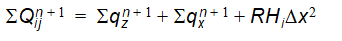
Equation 33.14

where - \(\sum q_{z}^{n+1}\) is the volumetric flow in vertical direction - \(\sum q_{x}^{n+1}\) is the volumetric flow in horizontal directions - R is the volumetric flow rate per unit volume from any sources and sinks - \(\Delta x\) is the spatial resolution in the horizontal direction - \(H_i\) is either the saturated depth for unconfined layers or the layer thickness for confined layers. See Figure 33.3 and Figure 33.4 for a description of the geometric relationships between the cells.

The horizontal flow components in Eq. (33.14) are given by

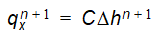
Equation 33.15

where - C is the horizontal conductance between any of the adjacent nodes in the horizontal directions.

The horizontal conductance in Eq. (33.15) is derived from the harmonic mean of the horizontal conductivity and the geometric mean of the layer thickness. Thus, the horizontal conductance between node i and node i-1 will be

Equation 33.16

where - KH is the horizontal hydraulic conductivity of the cell - Dz is the saturated layer thickness of the cell.

The vertical flow components in Eq. (33.14) are given by

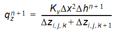
Equation 33.17

where - \(K_v\) is the average vertical hydraulic conductivity between nodes in the vertical direction, - \(\Delta_{i,j,k}\) and \(\Delta_{i,j,k+1}\) are the saturated thicknesses of layers k and k+1 respectively. For the average vertical hydraulic conductivity, \(K_V\), the SOR solver distinguishes between conditions where the hydraulic conductivity of layer k is greater than or less than the hydraulic conductivity of layer k+1. These cases are shown in Table 33.1 and Table 33.2.

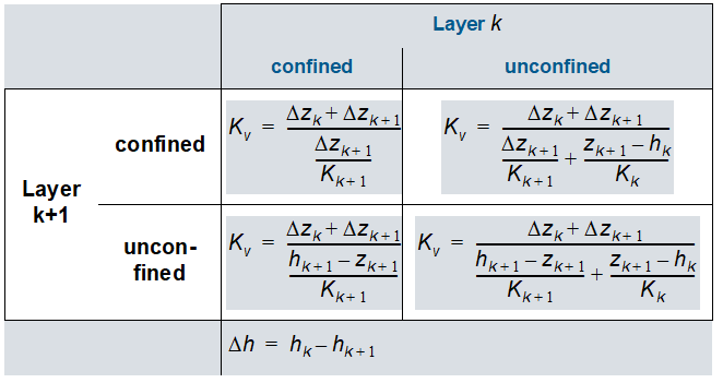
Table 30.1

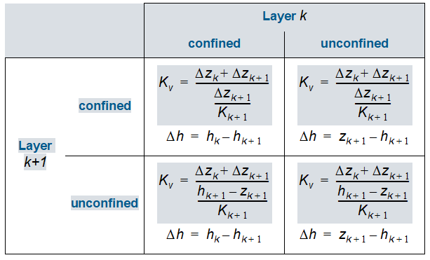
Table 30.2

The transient flow equation yields the finite difference expression

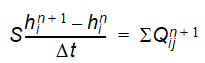
Equation 33.18

where - S is the storage coefficient - \(\Delta t\) is the time step. Eq. (33.18) is written for all internal nodes N yielding a linear system of N equations with N unknowns. The matrix is solved iteratively using a modified Gauss Seidel method (Thomas,1973).

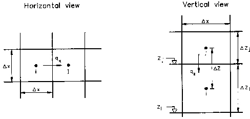
Figure 33.3 Spatial discretisation.

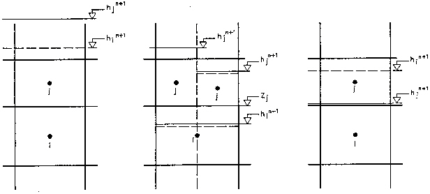
Figure 33.4 Types of vertical flow condition, a) confined conditions in nodes i and j,

b) unconfined condition in node i, c) unconfined in nodes i and j, d) dry conditions in node j and confined conditions in node i.

b. Relaxation Coefficient

The relaxation coefficient, w, is used in the solution scheme to amplify the change in the dependent variable (hydraulic head h) during the iteration. The value of w should be less than 2 to ensure convergence but larger than 1 to accelerate the convergence.

The optimal value is the value for which the minimum number of iterations are required to obtain the desired tolerance. It is a complex function of the geometry of the grid and aquifer properties. Figure 33.5 illustrates the relation between w and the number of iterations for a given grid. In practice the optimal value of w can be found after setting up the grid. The model is run for a few time steps (e.g. ten) with a range of w values between 1 and 2, and the total number of iterations is plotted for each run against the w value as shown in Figure 33.5. The minimum number of iterations corresponds to the optimal value of w.

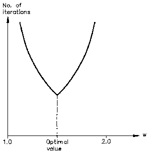
Figure 33.5 Empirically relationship between the relaxation coefficient w and number of iterations for a given model.

c. Maximum Residual Error

The maximum residual error is the largest allowable value of residual error during an iteration. The solution is obtained when the residual error during an iteration in any computational node is less than the specified tolerance.

The value of the maximum residual error should be selected according to aquifer properties and dimensions of the model. In practice, the maximum residual error value will always be a compromise between accuracy and computing time. It is recommended to check the water balance carefully at the end of the simulation, but it should be emphasized that large internal water balance errors between adjacent computational nodes may not be detected.

If large errors in the water balance are produced the maximum residual error should be reduced.

3. PCG Steady State Solver

The PCG Steady-State Solver is virtually identical to the transient PCG solver but has been implemented separately to enhance efficiency. In particular, experience has shown that different solver settings may be required when solving the system in steady state versus a transient solution. Furthermore, since the solvers have been implemented separately, there are a couple of options in the steady-state solver that are not available in the transient solver.

a. Average steady-state river conductance option

In the steady-state PCG solver, the conductance used for the SZ-river exchange in each iteration is averaged with the conductance of the previous iteration. This is done to reduce the risk of numerical instabilities when the conditions are changing between flow/no flow conditions in a computational cell. It is recommended to use this option, as it tends to enhance convergence.

b. Steady-state (constant) river water depth

When running a steady-state simulation that includes SZ-river exchange, a constant water depth may be specified for the river network, which can be used to calculate the head gradient driving the exchange flow.

If a constant river water depth is not specified, then the river water levels are determined in the following order

1. MIKE SHE hot-start water level if MIKE SHE hot-start is specified
2. Initial water levels from the river model if the river coupling is used
3. Water level equal to the river bed if not 1) or 2) - (i.e. dry river - no flow from the river to the aquifer).

4. Boundary Conditions

The SZ module supports the following three types of boundary conditions:

1. Head boundary - Dirichlet conditions, (Type 1) where the hydraulic head is prescribed on the boundary
2. Gradient boundary - Neumann conditions, (Type 2) where the gradient of the hydraulic head (flux) across the boundary is prescribed
3. Head-dependent flux - Fourier conditions, (Type 3) where the head dependent flux is prescribed on the boundary.

The head can be prescribed for all grid nodes (i.e. at the catchment boundary, as well as inside the model area) and for all computational layers. The head may be time-invariant equal to the initial head or can vary in time as specified by the user. An important option is the transfer of space- and time interpolated head boundaries from a larger model to a sub-area model with a finer discretisation.

Prescribed gradients and fluxes can be specified in all layers at the model boundary. Sinks and sources in terms of pumping or injection rates can be specified in all internal nodes. If the unsaturated zone component is not included in the model, the ground water recharge can be specified.

The exchange flow to the river system is included in the source/sink terms and can be regarded as a Type 3 boundary condition for cells with 'contact' to the river system. The exchange flow is a function of the water level in the river, the river width, the elevation of the riverbed, as well as the hydraulic properties at the riverbed and aquifer material.

a. Distribution of fluxes to the internal cells

Flux boundary, global specification

The total discharge of the actual time step (constant or time-varying) is distributed over the internal cells weighted by horizontal conductivity and full or saturated thickness (inflow/out-flow, respectively).

Inflow (positive discharge):

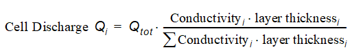
Equation 33.19

Outflow (negative discharge):

Same as above, but using actual saturated thickness instead of full layer thickness. In the case that all cells are dry the solution will switch to full layer thickness. However, in this case, the solution will be unstable anyway.

Flux boundary, distributed specification

The discharge is specified for each cell, separately for flow along the x- and the y-axis. It is applied to the adjacent internal cells as-is. If there are two internal cells along one axis then the in-/outflow will be distributed equally, without taking saturated thickness or conductivity into account. If there is no adjacent input cell along one axis then the specified flow will be disregarded with no warning. Flow can occur between an internal cell and all its adjacent boundary cells

Gradient boundary

Each cell receives a discharge calculated from the actual gradient (constant or time-varying), conductivity, cell size and saturated thickness. Positive gradient yields inflow:

\(Q = Gradient \cdot Conductivity \cdot CellSize \cdot Saturated thickness\)

Notes on Grid size

Distribution of actual cell discharges to the X- and Y- flow velocities are stored on the MIKE SHE result file, where they are needed for presentation and water balance extraction.

The X/Y-flow stored in a cell represents the flow from this cell to the neighbour cell in positive X/Y direction. The discharge of a cell in contact with more than one boundary cells of the actual boundary section is distributed as X/Y flow components to/from these boundary cells proportional to the grid size of the flow surfaces (constant in MIKE SHE).

Notes on the PCG solver

The discharges to/from the internal cells are updated at the start of each outer iteration and added to the “Right-Hand-Side” of the PCG solver. The discharges are distributed to the X/Y flow velocities (for results storing) at the end of each SZ time step.

Notes on the SOR solver

The discharges to/from the internal cells are updated at the start of each iteration and used as point source/sink terms in the solution. The discharges are distributed to the X/Y flow velocities (for results storing) at the end of each SZ time step.

5. SZ exchange with ponded water

The saturated zone component calculates the recharge/discharge between ponded water (OL) and the saturated zone (SZ) without the unsaturated zone, if the unsaturated zone is not included or if the phreatic surface is above the topography.

The exchange between SZ and OL is calculated implicitly using the Darcy equation

\(Q = \Delta h C_{1/2}\)

where - \(C_{1/2}\) is the conductance between the topography - the middle of the upper SZ calculation layer.

In the case of full contact between OL and SZ the conductance is calculated by

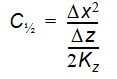
Equation 33.20

where - Dz is the thickness of layer 1 - Kz, is the vertical conductivity of layer 1.

In areas with reduced contact between overland and the saturated zone, the conductance between OL and layer 1 is calculated by

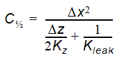
Equation 33.21

where - Dz is the thickness of layer 1 - \(K_Z\), is the vertical conductivity of layer 1 and \(K_{leak}\) is the specified leakage coefficient.

6. Saturated Zone Drainage

The MIKE SHE allows for flow through drains in the soil. Drainage flow occurs in the layer of the ground water model where the drain level is located. In MIKE SHE the drainage system is conceptually modelled as one 'big' drain within a grid square. The outflow depends on the height of the water table above the drain level and a specified time constant, and is computed as a linear reservoir. The time constant characterises the density of the drainage system and the permeability conditions around the drains.

The drainage option may not only be used to simulate flow through drainpipes, but also in a conceptual mode to simulate saturated zone drainage to ditches and other surface drainage features. The drainage flow simulates the relatively fast surface runoff when the spatial resolution of the individual grid squares is too large to represent small scale variations in the topography.

Drainage water can be routed to local depressions, rivers or model boundaries. See Groundwater drainage for further details about routing of drainage water.

There are also some additional Extra Parameter options for drainage routing:

• SZ Drainage to Specified River H-points
• SZ Drainage Downstream Water Level Check

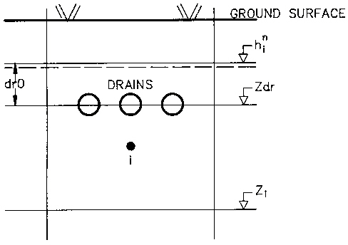
Figure 33.6 Schematic presentation of drains in the drainage flow computations.

a. SZ Drainage with the PCG solver

When the PCG solver is used, the drain flow is added directly in the matrix calculations as a head dependent boundary and solved implicitly, by

Equation 33.22

where - h head in drain cell, - \(Z_{dr}\) is the drainage level - \(C_{dr}\) is the drain conductance or time constant.

a. Drainage with the SOR Solver

When the SOR solver is used, drainage is only allowed from the top layer of the saturated zone model. In this case, the new water table position at the end of the time step is calculated from the flow balance equation

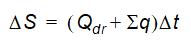
Equation 33.23

where - \(\Delta S\) is the storage change as a result of a drop in the water table, - \(Q_{dr}\) is the outflow through the drain - \(\sum q\) represents all other flow terms in a computational node in the top layer (i.e. net outflow to neighbouring nodes, recharge, evapotranspiration, pumping and exchange to the river etc.).

The change in storage per unit area can also be calculated from

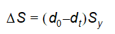
Equation 33.24

where - \(d_0\) is the depth of water above the drain at the beginning of the time step, - \(d_t\) is the depth of water above the drain at the end of the time step - \(S_y\) is the specific yield.

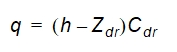
\(Q_{dr}\) is calculated based on the mean depth of water in the drain during the time step. Thus,

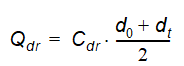
Equation 33.25

where - \(C_{dr}\) is the drain conductance or time constant.

Substituting (33.24) and (33.25)) into (33.23) and rearranging, the water depth at the end of a time step, dt, can be calculated by

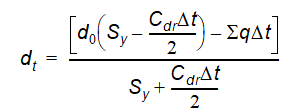
Equation 33.26

From which the new water table elevation, ht, at the end of the time step can be calculated by

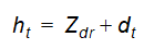
Equation 33.27

where - \(Z_{dr}\) is the elevation of the drain.

The drainage outflow is added as a sink term using the hydraulic head explicitly. The computation for drainage flow uses the UZ time step, which is usually smaller than the SZ time step. The initial drainage depth d0 at the beginning of an SZ time step is set equal to h - Zdr, where h is the water table elevation at the end of the previous SZ time step. d0 is adjusted during the sequence of smaller time steps so that a successive lowering of the water table and the outflow occurs during an SZ time step. This approach often overcomes numerical problems when large time steps are selected by the user. If the drainage depth becomes zero during the calculations drainage flow stops until the water table rises again above the drain elevation.

7. Initial Conditions

The initial conditions are specified in the Setup Editor and can be either constant for the domain or distributed, using .dfs2 or .shp files. The initial conditions in boundary cells are held constant during the simulation, which means that the initial head in cells with Dirichlet's boundary conditions is the boundary head for the simulation.

If there is ponded water on the ground surface at the start of the simulation and the simulation is steady-state, then the depth of ponded water is treated as a fixed head for SZ.

8. The Sheet Pile Module

The Sheet Piling module is an add-on module for the PCG groundwater (SZ) solver in MIKE SHE that allows you to reduce the conductance between cells in both the horizontal and vertical directions. Vertical sheet piling reduces the horizontal flow between adjacent cells in the x- or y-direction. It is defined by a surface with a specified leakage coefficient located between two MIKE SHE grid cells in a specified computational layer. If the Sheet Piling module is active, then the horizontal conductance, Ch, for flow between two cells is calculated as

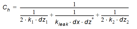
Equation 33.28

where - \(k_i\) is the hydraulic conductivity of the cells on either side of the sheet pile [L/T] - \(k_{leak}\) is the leakage coefficient of the sheet pile between the cells[1/L] - \(dz_i\) saturated layer thickness [L] - \(d_z\) maximium of dz1 and dz2 [L]

Similarly, reducing the vertical conductance between two layers can simulate a restriction in vertical flow (e.g. thin clay layer or liner). Thus, if the Sheet Piling module is active for vertical flow, the vertical conductance between two layers is calculated as

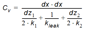
Equation 33.29

where - \(k_i\) is the hydraulic conductivity of the cells above and below the sheet pile [L/T] - \(k_{leak}\) is the leakage coefficient [1/T] - \(dz_i\) is the layer thickness [L].