Richards Equation
1. Overview
The driving force for transport of water in the unsaturated zone is the gradient of the hydraulic head, h, which includes a gravitational component, z, and a pressure component, \(\psi\). Thus,
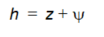
Equation 31.01
The gravitational head at a point is the elevation of the point above the datum (z is positive upwards). The reference level for the pressure head component is the atmospheric pressure. Under unsaturated conditions the pressure head, \(\psi\) is negative due to capillary forces and short range adsorptive forces between the water molecules and the soil matrix. These forces are responsible for the retention of water in the soil. As these two forces are difficult to separate, they are incorporated into the same term. Although the physical phenomena creating the pressure head under unsaturated and saturated conditions are very different, the pressure head is considered to be a continuous function across the water table, with the pressure being negative above and positive below the water table.
For vertical flow, the driving force for the transport of water is the vertical gradient of the hydraulic head. Thus,

Equation 31.02
The volumetric flux is then obtained from Darcy's law:
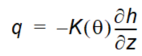
Equation 31.03
Where
- K(\(\theta\)) is the unsaturated hydraulic conductivity. Assuming that the soil matrix is incompressible and the soil water has a constant density, the continuity equation will be:
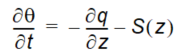
Equation 31.04
Where
- \(\theta\) is the volumetric soil moisture and S is the root extraction sink term.
Combining Eqs. (31.1),(31.3) and (31.4) yields

Equation 31.05
The dependent variables, \(\theta\) and \(\psi\) in Eq. (31.5) are related through the hydraulic conductivity function, K(\(\theta\)), and the soil moisture retention curve, \(\psi (\theta)\)
Eq. (31.5) is general, in the sense that it is equally valid in both homogeneous and heterogeneous soil profiles, and there are no constraints on the hydraulic functions.
Introducing the concept of soil water capacity

Equation 31.06
which is the slope on the soil moisture retention curve, then the tension- based version of Eq. (31.5) is

Equation 31.07
This equation is usually referred to as Richards equation, which is named after L.A. Richards who first used it in 1931. It still applies when \(\psi\) becomes positive, in which case the equation degenerates to the LaPlace equation.
The sink terms in Eq. (31.7) are calculated from the root extraction for the transpiration in the upper part of the unsaturated zone. The integral of the root extraction over the entire root zone depth equals the total actual evapotranspiration. Direct evaporation from the soil is calculated only for the first node below the ground surface.
2. Numerical Solution of Richards Equation
MIKE SHE uses a fully implicit formulation in which the space derivatives of Eq. (31.7) are described by their finite difference analogues at time level n+1. The values of \(C(\theta)\) and \(K(\theta)\) are referred to at time level n+½. These are evaluated in an iterative procedure averaging \(C^n\) , \(K^n\) with \(C^m\), \(K^m\) respectively. \(C^m\), \(K^m\) are calculated as a running average of the coefficients found in each iteration.
This solution technique has been found to eliminate stability and convergence problems arising from the non-linearity of the soil properties.
For an interior node, the implicit scheme yields the following discrete formulation of the vertical flow:

Equation 31.08
where the subscript J refers to the spatial increment and the superscript n refers to the time increment. The vertical grid system for a soil column is shown in Figure 31.1. Similar to Eq. (31.8) the discrete form of Eq. (31.1) gives
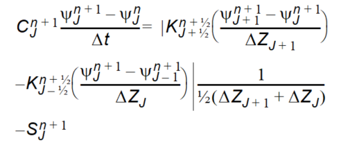
Equation 31.09
The soil property K is centred in space using the arithmetic mean:

Equation 31.10
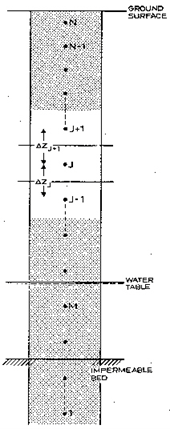
Figure 31.1 Vertical Discretisation in the Unsaturated Zone.
Eq. (31.9) involves three unknown values at time n+1 and one known value at time n for each node. Written for all nodes with reference to Figure 31.1, a system of N-M+1 equations with N-M+1 unknowns is obtained. The system of equations forms a tri-diagonal matrix:
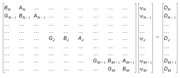
Equation 31.11
The J'th row in the matrix is

Equation 31.12
Where
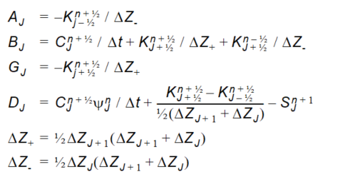
Equation 31.13
The solution to the matrix system Eq. (31.11) is solved by Gaussian elimination. Assuming that \(\psi_j^{n+1}\) and \(\psi_{j+1}^{n+1}\) can be related in the following recurrence relation

Equation 31.014
The \(E_{J+1}\) and \(F_{J+1}\) can be calculated by combining Eqs. (31.12) and (31.14) as follows:

Equation 31.15
Given the boundary conditions at the bottom and top nodes, \(\psi\) is computed for all nodes in a double sweep procedure:
- E and F values are calculated from Eqs. (31.13) and 31.15) for all nodes from bottom-to-top in a E, F-sweep.
- \(\psi\) is then calculated from Eq. (31.14) for all nodes in a top-to-bottom sweep.
Briefly, the iterative procedure within each time step is
-
the final result at time n (i.e.\(C_J^n\) and \(K_J^n\)) is used for the initial estimate of and for the first iteration
-
then the following convergence criteria is checked for every node after each iteration, i

Equation 31.16

Equation 31.17
-
if this convergence criteria is satisfied then a solution at the current time level (i.e. n+1) has been found.
-
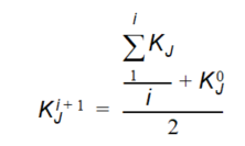
if the criteria is not fulfilled then \(C_J^{i+1}\) and \(K_J^{i+1}\) are updated for the next iteration by
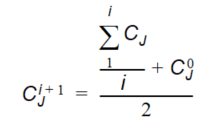
Equation 31.18
Equation 31.19
3. Boundary Conditions
The unsaturated zone extends from the ground surface to the groundwater table. The vertical flow is determined by the boundary conditions at each end of the column. However, the UZ column only exchanges water with the upper node of the SZ model, even if the UZ model extends below the top layer of the SZ model (see Limitations of the UZ - SZ coupling).
a. Upper boundary
The upper boundary condition is either
- a constant flux condition within each time step (Neumann boundary condition), which is determined by the infiltration rate, or
- a constant head condition within each time step (Dirichlet boundary condition), which is determined by the level of ponded water on the surface
If the infiltration is equal to the net rainfall rate at the soil surface, R, Eq. (31.9) can be written for the top node N as
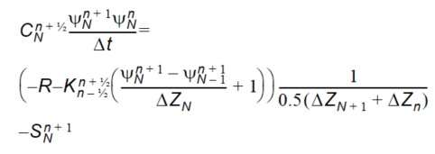
Equation 31.20
where R is defined negative downwards.
Writing Eq. (31.20) in a similar form to Eq. (31.12) yields

Equation 31.21
where
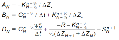
Equation 31.22
If water is ponded on the ground surface, the first node is assumed saturated and the boundary condition simply becomes
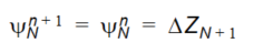
Equation 31.23
At the beginning of each UZ time step, the amount of available water for infiltration is calculated as the amount of ponded water, plus the net rainfall at the ground surface, minus evaporation from ponded water.
The upper boundary condition is applied depending on the deficit in the uppermost UZ node:
- If the available water exceeds the deficit in the top UZ node, then the head boundary is used.
- If the available water is less then the deficit in the top UZ node, then a flux boundary is used.
If the head boundary is used, then when the solution is found, the amount of infiltration is compared against the available amount of infiltration. If the available infiltration is exceeded then the solution is repeated with the flux boundary.
If the flux boundary is used, then the available water for infiltration is divided by the time step length to get the infiltration rate. When the solution is found, the water content in the uppermost UZ node is compared to the saturated water content. If the saturated water content was reached or exceeded, then the solution is repeated using the head boundary.
The solution is restricted to a maximum of one repeat in each time step, to prevent an infinite loop.
c. Lower Boundary
In most cases, the lower boundary is a pressure boundary that is determined by the water table elevation. Then Eq. (31.22) consists of N-M equations. If node M is the first node below the water table, then

Equation 31.24
where h is the distance between the water table and node M. Noted that \(\psi_M\) is independent of \(\psi_{M+1}\) since \(E_{M+1} = 0\).
If the UZ model is not coupled to a SZ model, then the lower boundary is automatically converted from a pressure head boundary to a zero flux boundary (Q=0) if the water table falls below the impermeable bed (see Figure 31.1) and, at same time there is an upward flux in the lower part of the profile. The head boundary is re-started as soon as a positive hydraulic pressure gradient is calculated or the water table starts to rise in the profile.
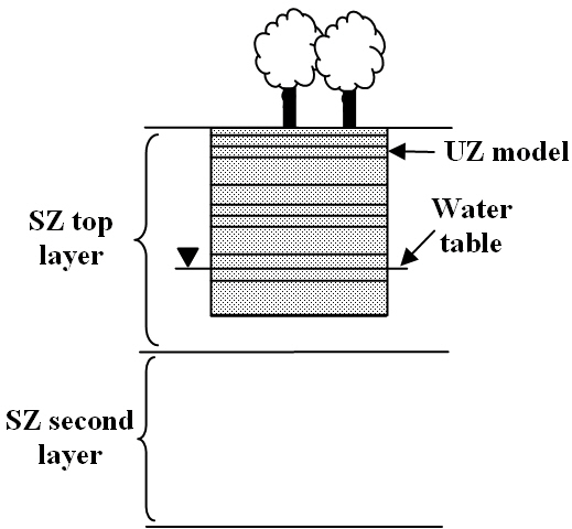
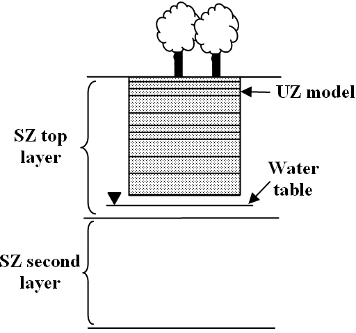
However, when the UZ model is coupled to an SZ model, the UZ model exchanges water only with the top node of the SZ model. This can lead to three principle conditions:
- If the UZ model intersects the water table in the top layer of the SZ model, then the lower boundary is a normal pressure boundary.
- If the UZ model does not extend to the bottom of the uppermost SZ layer, and the water table in the SZ model falls below the bottom UZ layer, then an error will be generated and the simulation will be stopped.
- If the UZ model extends below the top SZ layer and the top SZ layer dries out, then the UZ model treats the bottom boundary as either a pressure boundary with the pressure equal to the elevation of the bottom of the uppermost SZ layer, or a zero-flux boundary if there is an upward gradient at the lower boundary. The zero-flux boundary is only used for the Full Richards Equation option because the tension term can yield an upwards flow from the groundwater table, which is not physically possible when the upper SZ layer is dry.
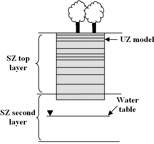
In the first and last cases above, the flux out the bottom of the UZ column is added as a flux boundary condition to the uppermost SZ node.
6. Initial Conditions
By default, the initial conditions for \(\psi\) are generated by MIKE SHE assuming an equilibrium soil moisture/pressure profile with no-flow. The equilibrium profile is calculated assuming hydrostatic conditions, as illustrated in Figure 31.2. The pressure decreases linearly from zero at the groundwater table to \(\psi{fc}\) when the moisture content reaches the field capacity and is then constant for all nodes above this point. The assumption is that the flow is (almost) zero at moisture contents below the field capacity.
The assumption that the initial water content is not below field capacity means that ET can occur from the first time step. If the water content was based on the saturation-pressure profile all the way to the residual water content, then the model would likely start with very dry soils. There would be no recharge or ET until the soils wetted up after significant rainfall.
However, in arid and semi-arid conditions the equilibrium water content may be quite low, as the soil profile may have drained for a long time with little infiltration. In this case, it is usually better to base the initial condition on the full saturation-pressure relationship - all the way to residual water content.
In both cases, an initial warm up of the UZ is usually required. In the first case, there will be some initial drainage from the UZ as the moisture content equilibrates with the rainfall rate. In the second case, the soil profile will gain water and the groundwater recharge will be initially very low as the soil profile absorbs all of the infiltration.
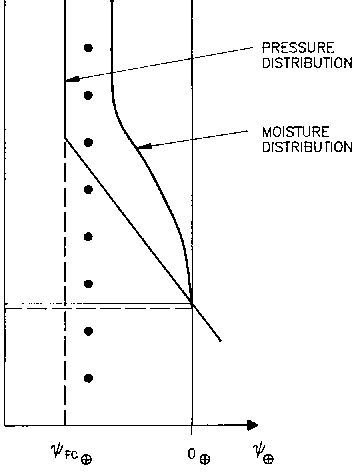
Figure 31.2 Illustration of initial soil moisture profile and pressure head profile.
7. Sources and sinks
There is a source/sink term for each computational node. These sink terms are calculated from the root extraction due to transpiration in the upper part of the unsaturated zone. The integral of the root extraction over the entire root zone depth equals the total actual evapotranspiration. Direct evaporation from the soil is calculated only for the first node in the soil column.