Overview of the UZ User Interface¶

The setup of the UZ model can be divided into two steps: The definition of the soil profile and the definition of the vertical numerical grid. These two steps are separate in the Gravity Flow and Richards Equation methods. In the Two-Layer UZ method the vertical discretisation is pre-defined (a root zone and area below the roots), so only the soil properties need to be defined.

1. Definition of the soil profile¶

Richards Equation and Gravity Flow¶

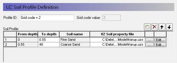
In the Gravity flow and Richards Equation methods, the soil profile section in the allows you to define the vertical soil profile.

Soil layers can be added, deleted and moved up and down using the icons.

From and To Depths refer to the distances to the top and bottom of the soil layer, below the ground surface. Only the To Depth item is editable, as the From Depth item is equal to the bottom of the previous layer.

Soil name is the name of the soil selected in the UZ Soil Property file. It is not directly editable but must be chosen from the list of available soil names when you assign the UZ Soil property file using the file browser.

UZ Soil property file is the file name of the soil database, in which the soil definition is available. The Edit button opens the specified Soil property database file, whereas the Browse button [...] opens the file browser to select a file. See UZ Soil Properties Editor.

Note

The depth of the soil profile does not have any influence on the calculation. The only constraint is that the soil profile must be deeper than the numerical grid.

If you specify multiple soils in a soil profile, then the infiltration through the column will depend on the effective hydraulic conductivity function associated with water content, K(). This means that zones of high saturation may build up within the soil column. Depending on the situation, this may or may not be realistic. The UZ columns do not communicate laterally with one another, so there is no way for such perched conditions to redistributed laterally to neighbouring cells.

In the case of Richards Equation, heterogeneous profiles can also lead to capillary barriers. This occurs when fine-grained soil is underlain by a coarser soil. In this case, capillarity will retain the water in the fine-grained soil because the gravity gradient is less than the capillary pressure holding the moisture in the fine-grained soil. This does not occur in the Gravity Flow method, because capillarity is ignored.

Two-Layer UZ method¶

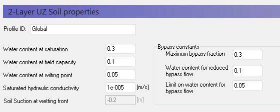
In the Two-Layer UZ method, only the soil properties need to be defined.

The soil properties are not defined from the Soils Editor, rather they must be input directly in the dialogue.

2. Definition of vertical UZ numerical grid¶

The Gravity and Richards Equation methods assume that the soil profile is divided into discrete computational nodes. The non-linearity of the unsaturated flow process creates large gradients in soil pressure and soil moisture content during infiltration. Therefore, it is important to select appropriate nodal increments, so as to describe the flow process with sufficient accuracy but at the same time keeping the computational time reasonable. This trade-off can become a key constraint in catchment-scale simulations.

Note

The UZ model only connects to the top layer of the SZ model. All nodes below the water table are ignored. All nodes below the bottom of SZ layer 1 are also ignored. However, results will be output at all of these nodes, which can lead to unnecessarily large output files. There is also a small memory overhead associated with the extra nodes, but the extra nodes cause very little computational overhead.

The simulation of Hortonian ponding at the ground surface (high rainfall intensity on dry, low permeable soil) requires a fine spatial resolution in the upper part of the profile (see Figure 32.3). Deeper in the profile the gradients are smaller and larger node increments can usually be selected. However, in the case of coarser grained soil, there may again be very high saturation gradients near the water table. Thus, as a general guideline, one should choose a finer spatial resolution in the top nodes.

The discretisation should be tailored to the profile description and the required accuracy of the simulation.

If the full Richards equation is used the vertical discretisation may vary from 1-5 cm in the uppermost grid points to 10-50 cm in the bottom of the profile.
For the Gravity Flow module, a coarser discretisation may be used. For example, 10-25 cm in the upper part of the soil profile and up to 50-100 cm in the lower part of the profile.

The vertical discretization is defined in the lower half of the soil profile dialogue.

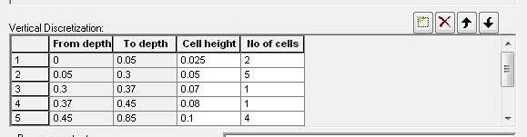
From and To Depths refers to the distances to the top and bottom of the soil layer, below the ground surface. Neither are directly editable since they are calculated from the number of cells and their thicknesses.

Cell Height is the thickness of the numerical cells in the soil profile.

No. of Cells is the number of cells with the specified cell height. Together these two values define the total thickness of the current section.

Note

The soil properties are averaged if the cell boundaries and the soil boundaries do not align.

Note

The boundary between two blocks with different cell heights, the two adjacent boundary cells are automatically adjusted to give a smoother change in cell heights.

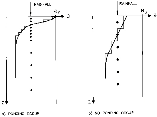
Figure 32.3 Examples of different increments in the soil profile and the resulting water content distribution of 1-3 cm for detailed studies and 3-5 cm for catchment studies. Further down in the profile larger increments can be chosen ranging from 10 cm to 30 cm.

Results¶

The UZ output contains all the information on pressure and saturation in the UZ columns, as well as information on the spatial processes, such as spatially distributed infiltration and groundwater recharge.

Gridded output items

The gridded output for the UZ solver is found in four files:

The output related to the 2 Layer Water balance method is found in the file projectname_wetland.dfs2. (The name reflects the earlier name of this module - the former wetland module).
The 2D results from the UZ model are found in two files: projectname_2- DUZ_AllCells.dfs2 and projectname_2DUZ_UzCells.dfs2. The 2D output includes output items related to spatial distribution of UZ processes, such as UZ-SZ exchange and groundwater recharge.
The 3D UZ outputs are found in projectname_3DUZ.dfs3. This file contains all the values in all the cells, such as the saturation in each UZ cell.

The detailed contents of these files are found in the Appendix: MIKE SHE Output Items.

Transient UZ column plot

One of the most interesting UZ outputs is the transient UZ column plot. The UZ in MIKE SHE is based on 1D columns. This plot displays the property (water content, pressure, etc.) of one column with depth versus time. This allows you to visualize, for example, the water content with depth at every saved time step in the simulation.

Evaluating the spatial distribution of UZ errors

The water balance program can be used to get an overview of the location and value of errors due to a poor setup of the unsaturated zone. Use the "Map output: Unsat. Zone Error" water balance type to produce a map of the error.

To further investigate problems with the UZ solver like water balance errors or excessive time step reductions there are two relevant grid output items:

UZ time step reduction count: After execution of the 1D UZ solver the resulting water balance will be checked. If the remaining error is too large (see "Maximum water balance error in one node" in UZ Computational Control Parameters) the solution will be discarded and restarted with a shorter time step. This could happen a couple of times in a row until an acceptable solution has been found. If there are problems with the setup though time steps can become too short, leading to an excessive run time. This output item can be used to identify the cells leading to the time step reductions. Note that the solver will stop processing new columns after the first column requires a restart. Due to the parallelization there can be a couple of cells signaling a restart at the same time, but not many more than the number of cores used, and usually not all columns will have been touched yet. So, there is no strict guarantee that the highest counts in the output contain the most problematic cells, but the probability is high.
UZ iteration count: This item contains the number of iterations leading to the accepted solution, averaged over the storing time step. If the time step has to be repeated with a shorter length, the iterations in the discarded time step will not be counted.