Finite Difference Method

The Finite Difference method is the most common method used in MIKE SHE. With the Finite Difference Method, you have the choice of two different numerical solvers. The SOR solver is an implicit matrix solver that is somewhat faster than the Explicit solver, but the increased speed is traded off for lower accuracy. Both are using the Diffusive Wave Approximation to the St Venant Equations.

1. Diffusive Wave Approximation

Using rectangular Cartesian (x, y) coordinates in the horizontal plane, let the ground surface level be zg (x, y), the flow depth (above the ground surface be h(x, y), and the flow velocities in the x- and y-directions be u(x, y) and v(x, y) respectively. Let i(x, y) be the net input into overland flow (net rainfall less infiltration). Then the conservation of mass gives

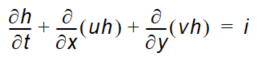
Equation 29.01

and the momentum equation gives

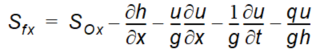
Equation 29.02

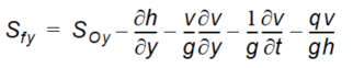
Equation 29.03

where - \(S_f\) is the friction slopes in the x- and y-directions - \(S_O\) is the slope of the ground surface. Equations (29.1), (29.2) and (29.3) are known as the St. Venant equations and when solved yield a fully dynamic description of shallow, (two-dimensional) free surface flow.

The dynamic solution of the two-dimensional St. Venant equations is numerically challenging. Therefore, it is common to reduce the complexity of the problem by dropping the last three terms of the momentum equation.

Thereby, we are ignoring momentum losses due to local and convective acceleration and lateral inflows perpendicular to the flow direction. This is known as the diffusive wave approximation, which is implemented in MIKE SHE.

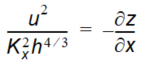
Considering only flow in the x-direction the diffusive wave approximation is

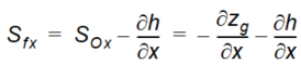
Equation 29.04

If we further simplify Equation (29.4) using the relationship z = zg + h it reduces to

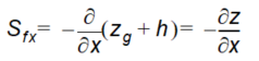
Equation 29.05

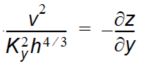
in the x-direction. In the y-direction Equation (29.5) becomes

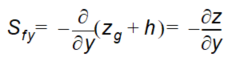
Equation 29.06

Use of the diffusive wave approximation allows the depth of flow to vary significantly between neighbouring cells and backwater conditions to be simulated. However, as with any numerical solution of non-linear differential equations numerical problems can occur when the slope of the water surface profile is very shallow and the velocities are very low.

Now, if a Strickler/Manning-type law for each friction slope is used; with Strickler coefficients Kx and Ky in the two directions, then

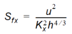
Equation 29.07a

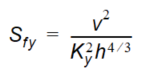
Equation 29.07b

Substituting Equations (29.4) and (29.5) into Equations (29.7a) and (29.7b) results in

Equation 29.08a

Equation 29.08b

After simplifying Equations (29.8a) and (29.8b) and multiply both sides of the equations by h, the relationship between the velocities and the depths may be written as

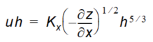
Equation 29.09a

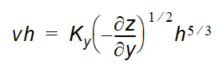
Equation 29.09b

Note that the quantities uh and vh represent discharge per unit length along the cell boundary, in the x- and y-directions respectively.

Also note that the Stickler roughness coefficient is equivalent to the Manning M. The Manning M is the inverse of the commonly used Mannings n. The value of n is typically in the range of 0.01 (smooth channels) to 0.10 (thickly vegetated channels), which correspond to values of M between 100 and 10, respectively.

2. Finite Difference Formulation

Consider the overland flow in a small region (see Figure 29.1) of a MIKE SHE model, having sides of length Dx and Dy and a water depth of h(t) at time t.

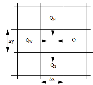
Figure 29.1 Square Grid System in a small Region of a MIKE SHE model

A finite-difference form of the velocity terms in Eq. (29.1) may be derived from the approximations

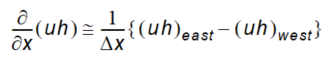
Equation 29.10

and

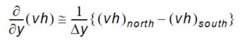
Equation 29.11

where the subscripts denote the evaluation of the quantity on the appropriate side of the square, and noting that, for example, Dx (uh)west is the volume flow across the western boundary

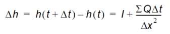
Equation 29.12

Equation 29.13

and where, i is the net input to overland flow in Eq. (29.1) the Q's are the flows into the square across its north, south, east and west boundaries evaluated at time t.

Now consider the flow across any boundary between squares (see Figure 29.2), where \(Z_U\) and \(Z_D\) are the higher and lower of the two water levels referred to datum. Let the depth of water in the square corresponding to \(Z_U\) be \(h_U\) and that in the square corresponding to \(Z_D\) to \(h_D\).

Figure 29.2 Overland flow across grid square boundary.

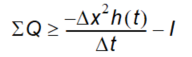
Equations (29.9a) and (29.9b) may be used to estimate the flow, Q, between grid squares by

Equation 29.14

where - \(K\) is the appropriate Strickler coefficient and the water depth, - \(h_u\), is the depth of water that can freely flow into the next cell. This depth is equal to the actual water depth minus detention storage, since detention storage is ponded water that is trapped in shallow surface depressions. Equation (29.14) also implies that the overland flow into the cell will be zero if the upstream depth is zero. The flow across open boundaries at the edge of the model is also calculated with Eq. (29.14), using the specified boundary water levels.

3. Successive Over-Relaxation (SOR) Numerical Solution

The method for solving the overland flow equations is similar to the method applied to the saturated zone flow. A linear matrix system of N equations with N unknown water levels is derived. The matrix is then solved iteratively, using the modified Gauss Seidel method. Because of the non-linear relationship

between water levels and flows, the 2nd order term is included in the Taylor series expressing the correction of water levels as a function of the residuals.

The flow is calculated for the remainder of any iteration using Eq. (29.14) whenever there is sufficient water in a cell, that is, whenever hu exceeds the minimum threshold that is specified by the user.

The exchange between ponded water and the other hydrologic components (e.g. direct exchange with the saturated zone, unsaturated infiltration, and evaporation) is added or subtracted from the amount of ponded water in the cell at the beginning of every overland flow time step.

Water balance correction

As the flow equations, so to speak, are explicit during one iteration, it is necessary to reduce the calculated flows in some situations to avoid internal water balance errors and divergence of the solution scheme.

Thus, requiring that the water depth cannot be negative, which implies that Dh ³ -h(t), rearranging Eq. (29.12) gives:

Equation 29.15

where - \(SQ\) is the sum of outflows and inflows.

Splitting SQ into inflows and outflows and remembering that outflow is negative, gives:

Equation 29.16

remembering that \(I = i \Delta x^2\) and i is the net input into overland flow (net rainfall less infiltration).

If necessary during an iteration, these calculated outflows are reduced to satisfy the equal sign of (29.16).

To ensure that the inflows, *\(SQ_{in}\), have been summed before calculating \(SQ_{out}\), the grid squares are treated in order of descending ground levels during each iteration.

4. Explict Numerical Solution

The explicit solution is different from the SOR solution in the sense that there is no iterative matrix solution. In other words, the exchange flows between every cell and to the river are simply calculated based on the individual cell heads. However, the explicit solution is much more restrictive in terms of time step. For the explicit solution to be stable, the flow must be slow relative to the time step. For example, a flood wave cannot cross a cell in one time step. So, this leads to the following 3-step calculation process for the explicit solution of the overland flow:

1. Calculate all flow rates and discharges between cells and between the overland cells and river links based on the current water levels
2. Loop over all the cells and calculate the maximum allowed time step length for the current time step, based on the following criteria
3. Courant criteria (see next section)
4. Cell volume criteria - the volume in the cell divided by the flow rate
5. River link volume criteria - the volume in the river link divided by the flow rate
6. River bank criteria - the exchangeable volume in the river link based on the river bank elevation divided by the flow rate

In most cases, the Courant criteria is the critical criteria for the maximum time step, with the Cell volume criteria sometimes being critical. The River link and River bank criteria are less commonly critical, but may become critical when the river is very shallow.

1. Calculate the actual flows between the all the cells and to/from the river links using the maximum allowed time step and update all the cell water depths.

5. Courant criteria

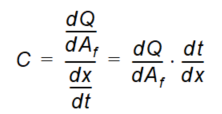
Courant number, C, represents the ratio of physical wave speed to the ‘grid speed’ and is calculated as

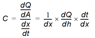
Equation 29.17

where - \(dQ\) is the change in flow rate, - \(dA\) is the change in cross-sectional area - \(dh\) is the change in water depth.

For a stable explicit solution the courant number must be less than one, which means that a wave cannot travel across a cell in less than one time step.

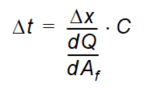
Solving for the time step, yields,

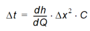
Equation 29.18

where - \(\Delta t\) is the time step - \(\Delta x\) is the cell width.

The differential term in (29.18) is the inverse of the derivative of the Mannings equation, (29.14), with respect to h, which goes to zero as the change in water depth approaches zero. Thus, flat areas with flat water levels will require very small time steps. Likewise, smaller grid spacing will also lead to smaller time steps.

6. Boundary conditions

The default outer boundary condition for the overland flow solver is a specified head, based on the initial water depth in the outer nodes of the model domain. Thus, if the water depth inside the model domain is greater than the initial depth on the boundary, water will flow out of the model. If the water depth is less than the initial depth on the boundary, the boundary will act as a source of water.

There is an Extra Parameter option that allows you to define a time varying outer boundary condition for Overland Flow. In this case, the outer boundary is still a fixed head boundary, but the fixed head is defined by a time-varying dfs2 file, instead of the initial water depth.

The boundary condition to the River can be calculated based on a Mannings resistance formulation, where the length is the distance from the node to the edge of the cell, the head difference is that between the cell and the River Link, and the depth of water is the depth above the detention storage.

The boundary condition to the river can also be calculated based on a standard weir formulation. The weir formulation must be used if two-way flow is calculated between the river and the cell.

In this case, the weir formula is a standard expression based on the Villemonte formula:

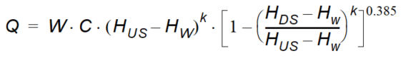
Equation 29.19

where - Q is the discharge over the weir, - W is the weir width, - C is the weir coefficient, - k is the weir exponent, - \(H_{US}\) is the upstream depth, - \(H_{DS}\) is the downstream depth - \(H_W\) is the crest level of the weir.

As the upstream water depth approaches zero, the flow over the weir becomes undefined. To prevent numerical problems, the flow is reduced linearly to zero when the water depth is below the user-defined minimum depth for full weir flow (assumes a triangular weir cross-section).

A minimum flow area threshold is defined to reduce numerical issues with small volumes of transfer from the river to the floodplain, The flow area is calculated by dividing the volume of water in the Coupling Reach by the length of the Coupling Reach. If the calculated area is less than the minimum flow area, then overbank spilling from the river is excluded.

Note

The minimum flow area threshold could unduly restrict overbank spilling if you have a long Coupling Reach and a small river section where overbank spilling occurs.

7. Low gradient damping function

In flat areas with stable ponded water, both the flow gradient and the water depth difference between grid cells will be zero or nearly zero. Equation (29.18) implies that as dh goes to zero \(\Delta t\) also goes to zero. To allow the simulation to run with longer time steps and dampen any numerical instabilities in areas with very low lateral flow, the calculated intercell flows are multiplied by a damping factor when the flow gradient between cells is close to zero.

Essentially, the damping factor reduces the flow between cells. You can think of the damping function as an increased resistance to flow as the flow between cells goes to zero. In other words, the flow goes to zero faster than the time steps goes to zero. This makes the solution more stable and allows for larger time steps. However, the resulting intercell flow will be lower than that calculated using the Mannings equation in the affected cells and neighbouring water levels will take longer to equilibrate. At very low flow gradients this is normally insignificant, but as the flow gradient increases the differences could become noticeable. Therefore, the damping function is only applied below a user-defined flow gradient.

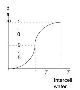
Figure 29.3 Default damping function for numerical stability at low gradients

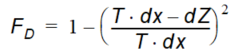
The default damping function is a pair of parabolic equations (see Figure 29.3). When the flow gradient between cells reaches the threshold the following damping function is applied

Equation 29.20

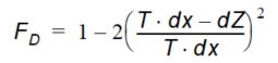
where - \(T\) is the user-specified threshold gradient, - \(dx\) is the cell size - \(dZ\) is the water level difference between the two nodes. When the water level difference reaches T dx/2, the damping function changes to

Equation 29.21

which goes to zero as the water level difference goes to zero.

In the log-log graph in Figure 29.4, you can see that the lateral flow betwen cells drops off very quickly when the Threshold is active. For example, if the difference between the surface water gradient and the Threshold gradient is 0.1, then the actual flow will only be 2% of the original flow. If the difference is 0.01, then overland flow will be essentially turned off between cells.

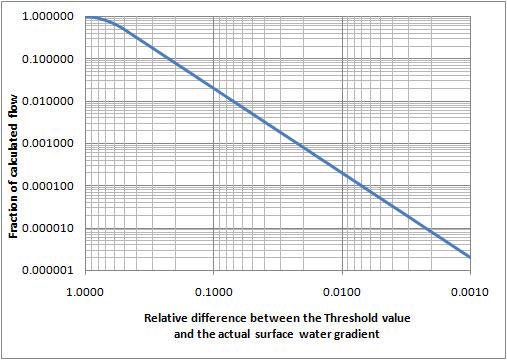
Figure 29.4 Actual overland flow as a function of the difference between the threshold gradient and the surface water gradient based on Equations (29.20) and (29.21).

Alternative damping function

An alternative damping function is available as an Extra Parameter that goes to zero more quickly and is consistent with the function used in the MIKE+ 2D Overland module.

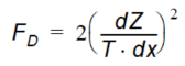
The alternative function is a single parabolic function (see Figure 29.5)

Equation 29.22

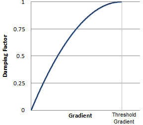
Figure 29.5 Alternative damping function activated by an Extra Parameter.

To activate the alternate function, you must specify the Alternative low gradient damping function boolean parameter in the Extra Parameters dialog .

For both functions and both the explicit and implicit solution methods, each calculated intercell flow in the current timestep is multiplied by the local damping factor, FD, to obtain the actual intercell flow. In the explicit method, the flow used to calculate the courant criteria are also corrected by FD.

The damping function is controlled by the user-specified threshold gradient (see Common stability parameters for the Overland Flow), below which the damping function becomes active.

8. Overland drainage

The amount of runoff generated by MIKE SHE depends on the density of the stream network in the river model. If the stream network is dense, then you will get more runoff in the model because the lateral travel time to the streams will be short, and the infiltration and evaporation losses will be smaller.

The Overland drainage function has been designed to facilitate a flexible definition of storm water drainage in both natural and urbanized catchments. In particular, the Overland drainage function supports the following features:

• In urban areas, paving and surface sealing (e.g. roof tops) limits infiltration and enhances runoff.
• Ponded water and precipitation are routed to user-defined locations (boundaries, depressions, manholes and streams).
• The time varying storage in the drainage system is accounted for by different inflow and outflow rates.
• Drainage rates can be controlled by drain levels, drainage time constants and maximum flow rates.
• Drainage is restricted if the destination water level is higher than the source water level.
• Urban development over time can be simulated by time varying drainage parameters.
• Infiltration and overland flow are calculated normally for ponded water that does not drain in the current time step.

Conceptually, the overland drainage function is shown in Figure 29.6.

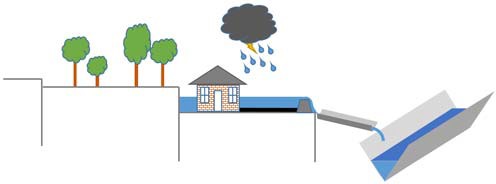
Figure 29.6 Conceptualization of the overland drainage function

Calculation Order and time step

The overland drainage is calculated explicitly in a particular order with respect to the other hydrologic processes. However, the exact order depends on what UZ solver is being used. In all cases interception is calculated first. When using the Richards- or the gravity-solver, ET will be calculated before OL drainage, when using the 2-layer UZ solver ET will be calculated after drainage.

After the drainage calculation any remaining precipitation will be added to the remaining ponded water.

If there is any ponded water remaining on the cell after the drainage has been removed, then it will be subject to other processes in the following order:

1. Infiltration to the unsaturated zone;

2. If the groundwater table is at/above ground: direct OL SZ exchange and

3. Finally, Lateral Overland Flow will be calculated to the adjacent cells.

The overland drainage is calculated for every cell independently. That is, the drainage that is calculated is not added to the destination cells until the end of the calculation for all the cells. This prevents circular drainage, and means that the order in which the calculation occurs is not relevant. After the overland drainage is calculated, the water depths in all the cells are updated - both sources and destinations. The calculation of infiltration and lateral OL flow is based on the updated ponded depths.

Although overland drainage is a fast process occurring at a time scale similar to overland flow itself, it is being calculated on the unsaturated zone time step that usually is significantly longer than the OL time step. The reasons for this are

1. The computational effort is lower

2. This ensures a more realistic share of the precipitation between infiltration and runoff. Overland drainage is being calculated after net rainfall, but before infiltration, so it can remove the appropriate amount of water from the system. If it was run with the overland component instead, the unsaturated zone component would process all net rainfall, leading to an overestimation of infiltration. Dividing the precipitation between drain inflow and the other processes does also to a certain degree depend on the length of the UZ time step. The length of the UZ time step during rain events can be controlled using the Precipitation-dependent time step control parameters (see Controlling the Time Steps).

Calculation method

The calculations of flow from ponding/precipitation into the overland drain storage and the flow from the drain storage to a recipient are very similar. They follow a linear reservoir type of equation, the flow is driven by a head difference and inhibited by a resistance, expressed as the in-/outflow time constants.

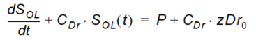
For flow into the drain the OL ponded storage change equals the difference between flow into OL and OL flow into the drain:

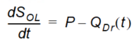
Equation 29.23

Where - \(SOL\) is the OL ponded storage, - \(P\) is net precipitation (the only source to OL considered for this purpose) - \(QDr\) is the flow into the drain. The flow into the drain is proportional to the drainable part of the current ponded volume, the proportion is given by the drain time constant:

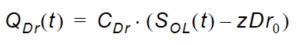
Equation 29.25

where - \(C_{Dr}\) is the drain time constant - \(zDr_0\) is the drain base level, i. e. the bottom level of the drainable part of OL storage. The drain base level will be the highest of a) ground surface, b) drain level, c) detention storage level (which by default is not drainable) and d) water level in the drain (only if option "check water levels" is active). Substituting (29.24) into (29.23) yields:

Equation 29.17

Further integrations and substitutions lead to the linear reservoir type of equation for the volume added to the drain:

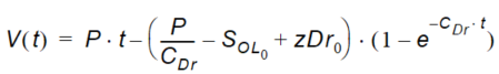
Equation 29.26

With \(S_{OL_0}\) being the initial overland storage.

In cases where the OL water level falls below or rises above the threshold for drain flow (the drain base level, see above) during a time step, drain inflow will only be calculated for the part of the time step where the threshold is exceeded.

Finally, the runoff coefficient and the maximum flow rate (if specified) will be applied.

Flow out of the drain to the recipient will be calculated in the same way, except there is no handling of cases where only part of the time step produces drain outflow. Because of this, when the recipient water level is above the drain water level, a reverse flow from the recipient into the drain would be calculated. If this happens the flow will be set to zero to prevent any reverse flow.

For drain inflow, if the option "Instantaneous drain inflow from net rainfall" is selected, the calculation will be simplified to

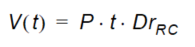
Equation 29.27

Where - \(Dr_{RC}\) is the user specified overland drainage runoff coefficient.

Constraints

Several constraints have been added to the formulation to make the overland Drainage function more practical.

• Paved Area Fraction - a paved fraction for the cell is used to reduce infiltration in urban areas.
• Runoff Coefficient - a fraction for the cell is used to partition the cell into a fraction that can drain to the drainage network, and a fraction where all rainfall and ponding is left to be subject to infiltration and finite difference Overland Flow. Note that the sub-cell volumes are not being tracked separately - subsequent components as well as subsequent drainage time steps will still work on the overall ponded water. So, this makes most sense if all the water is removed by infiltration or OL flow.
• Detention storage - the Ponded Drainage will only affect the depth of ponding above the Detention storage. However, this can be changed by means of an Extra Parameter.
• Drain Level - the Ponded Drainage will occur only when the ponded depth exceeds the Drain Level because the drain level is considered to be the bottom of the drain storage.
• Maximum drain inflow rate - a maximum drainage rate ensures that culvert capacities are not exceeded
• Check water levels - there is an optional check to include the destination water level in the calculation (for flow into the drain this is the drain water level, for flow out of the drain this is the recipient water level). If the downstream drainage destination does have a higher water level than the drain, then there will be no flow at all.
• Inflow time constant - the rate of inflow to the drains is controlled by a time constant/leakage factor.
• Outflow time constant - the rate of outflow to the destination is controlled by a time constant. If the outflow time constant is very small, then water may accumulate on a cell-by-cell basis in the “drain” (unless the ‘check water levels’ option is active). There is currently no limit on the amount of water that can accumulate in the drain.

Reference Drainage System

The Reference System for linking drainage source and destination is calculated by the Pre-Processor. By default, the drainage reference system is calculated downhill until either a local depression is found, or a stream or local boundary is encountered.

Optionally, the drainage can be routed to specified river nodes, or sewer manholes.

9. Multi-cell Overland Flow Method

The resolution of available topography data is often greater than the practical discretization of the overland flow model. This means that important topographic detail is often neglected in the overland flow model. The multi-cell overland flow method attempts to mitigate this discrepancy.

In the Multi-cell overland flow method, high resolution topography data is used to modify the flow area used in the St Venant equation and the courant criteria. The method utilizes two grids - a fine-scale topography grid and a coarser scale overland flow calculation grid. However, both grids are calculated from the same reference data - that is the detailed topography digital elevation model.

In the Multi-cell method, the principle assumption is that the volume of water in the fine grid and the coarse grid is the same. Thus, given a volume of water, a depth and flooded area can be calculated for both the fine grid and the coarse grid. See Figure 29.7.

In the case of detention storage, the volume of detention storage is calculated based on the user specified depth and OL cell area.

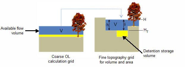
Figure 29.7 The constant volume from the coarse grid is transfered to the fine scale grid.

According to the Gauckler-Manning-Strickler formula, overland sheet flow can be expressed as

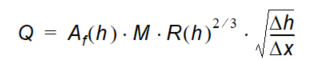
Equation 29.28

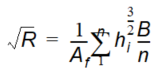
Where - \(Af\) is the flow area, - \(M\) is the Manning number, - \(h\) is the water depth, - \(\Delta x\) is the grid size - \(R\) is the hydraulic radius which, for practical reasons, is replaced by the resistance radius in the multi-cell method. Thus,

Equation 29.29

which expands to

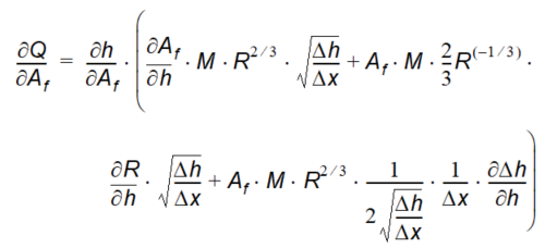
Equation 29.30

For any cross-section of flow, the resistance radius is calculated by

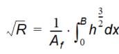
Equation 29.31

where again - \(h\) is the local water depth - \(B\) is the total width of the crosssection.

Thus, in a cross-section divided into n equal sub-grids,

Equation 29.32

where - \(h_i\) is the local water depth in each sub-grid. Since, Af is equal to

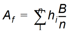
Equation 29.33

The resistance radius can be simplified to

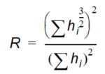
Equation 29.34

However, since parts of the sub-section may be dry, or the entire depth may not be available for flow because of detention storage, the actual resistance radius in the cross section is

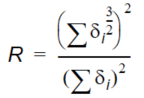
Equation 29.35

Where

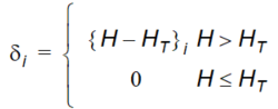
Equation 29.36

in which H is the water level in the refined cross-section and \(H_T\) is the maximum of the topography and level of detention storage in the current sub-grid.

Now, we need to apply the above formulation to a 2D coarse grid cell. In this case, the flow area and resistance radius is an average of the values along each row and column in the cell.

Thus, from Equation (29.33), the flow area for the x and y flow directions for each coarse grid cell is

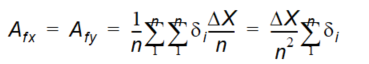
Equation 29.37

and from Equation (29.35), the resistance radius for the x and y flow directions for each coarse grid cell is

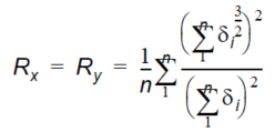
Equation 29.38

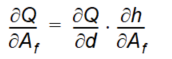
Finally, the courant criteria also includes the flow area. Thus, from Equation

Equation 29.39

which implies that the maximum allowed time step, \(\Delta t\),when using the multigrid method is

Equation 29.40

where

• \(\Delta x\) is the coarse overland flow grid size, the denominator is defined by Equation (29.30),
• C is the user-specified courant criteria.

Implementation and Limitations

When using the multi-cell overland flow method, each overland flow cell is divided into an integer number of sub-grid cells (e.g. 4, 9, 16, 25, etc). The elevation of the coarse grid nodes and the fine grid nodes are calculated based on the input data and the selected interpolation method. However, the coarse grid elevation is adjusted such that it equals the average of the fine grid nodal elevations. This provides consistency between the coarse grid and fine grid elevations and storage volumes. Therefore, there may be slight differences between the cell topography elevations if the multi-cell method is turned on or off. This could affect your model inputs and results that depend on the topography. For example, if you initial water table is defined as a depth to the water table from the topography.

Overland flow exchange with rivers does not consider the multi-cell method. That is, flow into and out of the River Links is controlled by the water level calculated from the elevation defined in the coarse grid cell. Likewise the flow area for exchange with the river is calculated as the coarse water depth times the overall grid size. Also, the elevation used when calculating flood inundation with flood codes only considers the average cell depth of the coarse grid.

However, if you choose to modify the topography based on a bathymetry file, or the river cross-sections, then this information will be used when calculating the multi-cell elevations.

Evaporation is adjusted for the area of ponded water in the coarse grid cell. That is, evaporation from ponded water is reduced by a ponded area fraction, calculated by dividing the area of ponding in the fine grid cell by the total cell area.

Infiltration from ponded water to the underlying UZ column or exchange between SZ and OL does not consider the multi-cell elevations. In both of these cases, only the average coarse grid elevation is used.