Coupling the Unsaturated Zone to the Saturated Zone
1. Overview
Briefly, the interaction between the unsaturated and saturated zones is solved by an iterative mass balance procedure, where the lower part of the unsaturated node system may be solved separately in a pseudo time step, between two real time steps. This coupling procedure ensures a realistic description of the water table fluctuations in situations with shallow soils. Particularly in these cases it is important to account for a variable specific yield above the water table, as the specific yield depends on the actual soil moisture profile and availability of that water.
The recharge to the groundwater is determined by the actual moisture distribution in the unsaturated zone. A correct description of the recharge process is rather complicated because the water table rises as water enters the saturated zone and affects flow conditions in the unsaturated zone. The actual rise of the groundwater table depends on the moisture profile above the water table, which is a function of the available unsaturated storage and soil properties, and the amount of net groundwater flow (horizontal and vertical flow and source/sink terms).
The main difficulty in describing the linkage between the two the saturated (SZ) and unsaturated (UZ) zones arises from the fact that the two components (UZ and SZ) are explicitly coupled (i.e., run in parallel) and not solved in a single matrix with an implicit flux coupling of the UZ and SZ differential equations. Explicit coupling of the UZ and SZ modules is used in MIKE SHE to optimize the time steps used and allows use of time steps that are representative of the UZ (minutes to hours) and the SZ (hours to days) regimes. MIKE SHE overcomes problems associated with the explicit coupling of the UZ and SZ modules by employing an iterative procedure that conserves mass for the entire column by considering outflows and source/sink terms in the saturated zone.
Error in the mass balance originates from two sources; 1) keeping the water table constant during a UZ time step and 2) using an incorrect estimate of the specific yield, Sy (the difference between the moisture content at saturation, \(\theta_s\), and moisture content at field capacity, \(\theta_{fc}\)) in the SZ-calculations. This is illustrated in Figure 31.4a. If outflow from the SZ is neglected, it appears from the figure that during the time n to n+m, the column has lost \(V_1\) mm of water (the light grey shaded area) and gained \(V_2\) mm (the dark shaded area).
The changes calculated by the UZ module for the areas \(V_1\) and \(V_2\) represent a redistribution of water in the unsaturated zone to obtain an equilibrium moisture profile within the soil column. Comparing the equilibrium moisture content and the moisture content at UZ time n in Figure 31.4 a shows that the moisture content is too high in the upper portions of the soil column. This should result in downward flow in the unsaturated zone, loss of soil moisture in area V1, increased soil moisture in area \(V_2\), and a rise in the water table. However, the SZ module uses a constant specific yield (Sy) defined for each grid cell in each calculation layer. On the other hand, the UZ can have a unique Sy value for each UZ node, which may differ from the Sy value used by the SZ. Thus, mass balance errors can occur in exchange calculations between the two modules. A mass-conservative solution is achieved by using a step-wise adjustment of the water table and recalculation of the UZ solution until the area of V1 and V2 are equal (see Figure 31.4b).
The procedure to deal with this mass balance error consists of a bookkeeping of the accumulated mass balance error, Ecum, for each UZ column and the upper SZ calculation cell associated with the column on a cell-by-cell basis. If |Ecum| exceeds a user specified value, Emax, the UZ coupling correction procedure corrects the water table of the upper SZ cell (i.e., the lower boundary condition for the UZ).
The correction procedure of step-wise water table adjustments and additional UZ calculations is repeated until |Ecum|is less than Emax for each column that has failed the Emax criteria. During this correction procedure, the UZ module of MIKE SHE operates on a copy of the water table solution for the upper SZ calculation layer. After each SZ time step the UZ copy is updated with the new water table from the SZ solution and then adjusted during the succeeding UZ time step(s) until the next SZ time step. The calculated adjustments are converted to an additional flux term (multiplied with the specific yield of SZ and divided by the SZ time step length) and added to the uncorrected UZ- to-SZ flux term. The corrected UZ-to-SZ flux term is used by the SZ module as an explicit source/sink term during the next SZ time step.
The size of Emax determines the largest allowable mass balance before adjustments are made. Typically, an Emax value between 1-2 mm is an appropriate choice for regional MIKE SHE simulations. The Emax value is specified in the [UZ Computational Control Parameters) dialogue.
2. Steps in the Coupling Procedure
The following outlines the actual steps in the coupling procedure used for each UZ time step:
- If the total water content above the datum \(Z_o\) (\(Z_o\) should always be lower than the lowest elevation of the water table) is designated \(W^n\), the flow rate across the lower boundary in UZ-time step n to n+1 is
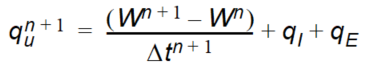
Equation 31.36
where - \(W^{n+1}\) =the new water content; - \(q_I\) = the infiltration rate (negative downwards); - \(q_E\) = the evapotranspiration loss. (Note: negative values of qu indicate downward flow). 2. Assuming that the groundwater outflow in a cell is steady, the accumulated error at UZ time n+1 is:
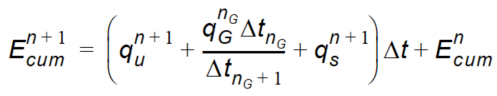
Equation 31.37
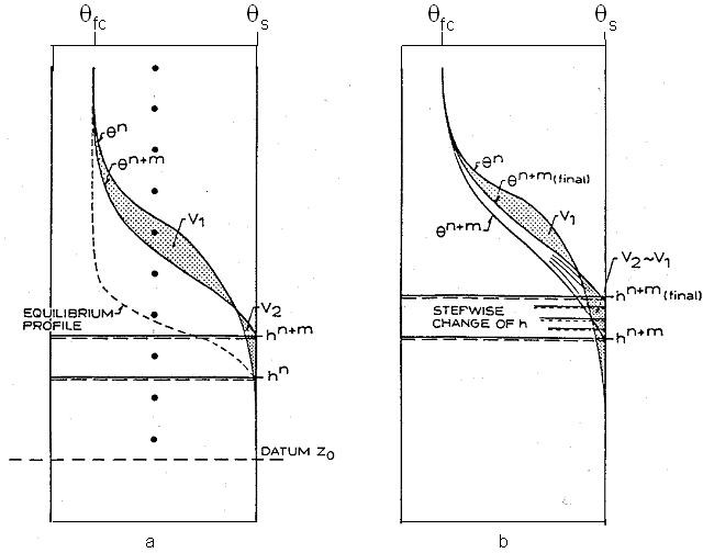
Figure 31.4 a) Soil moisture content at two times n and n+m without corrections, and b) Soil moisture content at time n+m before and after correction.
where - \(q_g^{n_g}\) (positive outwards) is the sum of the groundwater outflow rate for the cell in the last groundwater time step (\(n_G\)) scaled to the new SZ time step length (\(n_g+1\)) and \(q_s^{n+1}\) (positive outwards) is the sum of source sink terms calculated by the UZ module for the current time n+1 (e.g., stream/aquifer exchanges, irrigation).
It should be noted that if \(E_{cum}\) is less than zero there is a deficit of water stored in the column and if \(E_cum\) is greater than zero there is an excess of water stored in the column.
-
If \(\lvert E_{cum}^{n+1} \rvert\) less than \(E_{max{\) corrections are not made for the current UZ time step.
-
If \(\lvert E_{cum}^{n+1} \rvert\) exceeds \(E_{max{\) the following corrections are made:
a. IF \(\lvert E_{cum}^{n+1} \rvert\) is negative or positive, the water table is raised or lowered, respectively, in prescribed increments that depend on the distance between UZ nodes and the UZ-calculation in time step n to n+1 is repeated as described above.
b. In the Full Richards solution the UZ flow solution is repeated4for the last three nodes above the water table to reduce numerical overhead. In the Gravity Flow option, the UZ flow solution is repeated for the entire column. The UZ flow solution is not repeated for the two-layer UZ option.
c. The change in water volume \(W^{n+1*}\) over the entire column is computed and a new \(\lvert E_{cum}^{n+1} \rvert\) is calculated.
d. If \(\lvert E_{cum}^{n+1} \rvert\) is less than \(a \cdot E_{max}\), where a is a hard-coded correction factor equal to 0.9, the error associated with the solution is considered acceptable and the procedure stops. If \(\lvert E_{cum}^{n+1} \rvert\) is greater than or equal to \(a \cdot E_{max}\), the solution is unacceptable and steps a) through d) are repeated until criteria d) is satisfied. The value a defines a threshold for stopping the procedure lower than that used to initiate the procedure, which prevents correction overshoots.
e If \(\lvert E_{cum}^{n+1} \rvert\) changes sign the solution is considered acceptable and he procedure stops. The adjustment required to obtain a value of zero is calculated using a secant line approach. n + 1 cum
- A new recharge rate, \(q_u^{n+1*}\) is calculated taking the adjustments into account.
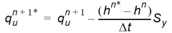
Equation 31.38
where - \(h^{n*}\) is the new water table elevation after step d) calculated by the UZ module - \(\Delta t\) is the length of the current UZ time step (n+1). If SZ outflows for the next SZ time step (\(n_G+1\)) are unchanged, the water table from the SZ calculation will be \(h^{n+1}=h^{n*}\) calculated in the last UZ time step before an SZ time step (see Eq. (31.38)).
If \((h^{n*}-h^n)S_y / \Delta_t > q_{max}\), where \(q_{max}\) is a maximum infiltration rate the corrected rate is reduced to \(q_{max}\). In the Richards Equation and Gravity Flow options \(q_{max}\) is \(0.7K_s\) and \(0.4K_s\) for rising and falling water table conditions, respectively, where \(K_s\) is the saturated hydraulic conductivity of the UZ node at the water table. In the Two-layer UZ option, the infiltration rate is used to constrain the corrected rate.
Steps 1-5 are repeated for all UZ time steps within each SZ time step. The flows are accumulated and passed as an average rate, \(q_u\), for the next SZ time step. The average \(q_u\) is used as a flux boundary condition in the SZ differential equations.