The MIKE SHE User Interface¶

The MIKE SHE user interface is organized by task. In every model application you must

Set up the model,
Run the model, and
Assess the results.

The above three tasks are repeated until you obtain the results that you want from the model.

When you create or open a MIKE SHE model, you will find yourself in the Setup Tab of the MIKE SHE user interface.

The following sections provide a quick overview of the main hydrologic processes in MIKE SHE. For more detailed information on the individual parameters, see Setup Data Tab.

Alternatively, this manual also contains detailed user guidance and information in the sections:

1. The Setup Editor¶

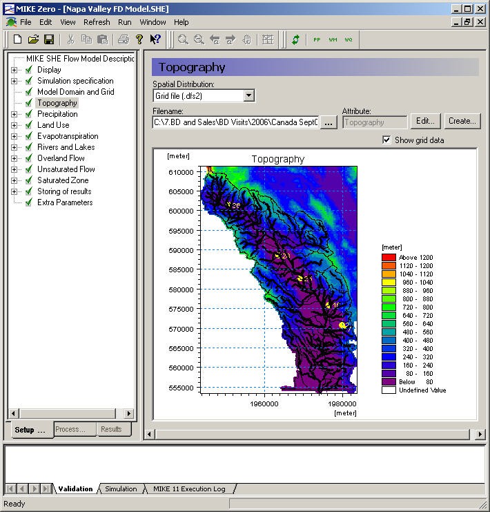
Figure 2.1: Graphical overview of the topography in the MIKE SHE GUI, without the Project Explorer.

The Setup editor is divided into three sections - the data tree, a context sensitive dialogue and a validation area.

The data tree is dynamic and changes with how you set up your model. It provides an overview of all of the relevant data in your model. The data tree is organized vertically, in the sense that if you work your way down the tree, by the time you come to the bottom you are ready to run your model.

The context sensitive dialogue on the right allows you to input the required data associated with your current location in the data tree. The dialogues vary with the type of data, which can be any combination of static and dynamic data, as well as spatial and non-spatial data. In the case of spatial and time varying data, the actual data is not input to the GUI. Rather, a file name must

be specified and the link to the file is stored in the GUI. Furthermore, the distribution of the data in time and space need not correspond between the various entries. For example, rainfall data may be entered as hourly values and pumping rates as weekly values, while the model may be run with daily time steps.

In addition to the data tree the main MIKE SHE menu also provides you with an overview of some of the standard parameters specific to your model. The parameters displayed depend on the options selected in the Simulation specification in the data tree. The table not only provides an overview of the key parameters but also provides a quick way of modifying the input parameters without having to go through the data tree. Overviews of module specific parameters are also available in the main menus of the Land Use, Overland Flow and the Saturated Zone modules. The model parameters can either be displayed in the same order as in the data tree (the default option) or by parameter. The Sort by Parameter option groups layered items by parameter, for example the horizontal conductivity or lower levels.

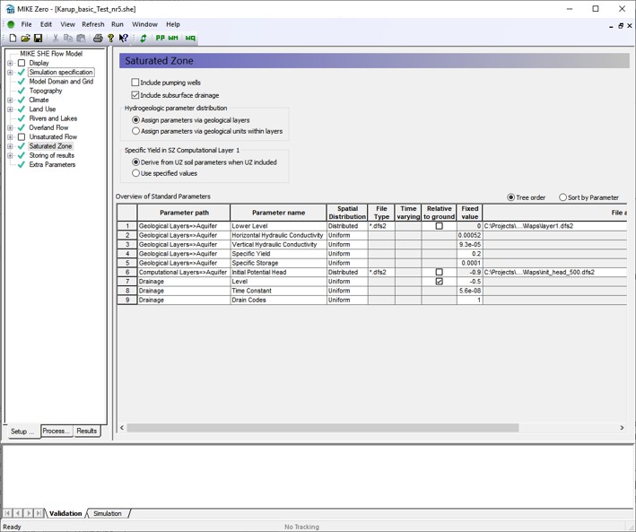
Figure 2.2 Example of Overview of Standard Parameters in the Saturated Zone dialogue in the MIKE SHE GUI.

The validation area at the bottom of the dialogue provides you with immediate feedback on the validity of the data that you have input.

After you have set up your model, you must switch to the Processed Data tab and run the pre-processing engine on the model. This step reconciles all of the various spatial and time series data and creates the actual data set that will be run by MIKE SHE. Once the data has been pre-processed the simulation can be started. Using the Pre-processing tab at the bottom, you can view the pre-processed data.

After the simulation is finished, you can switch to the Results tab, where you can view the detailed time series output as in a report-ready HTML view.

Alternatively, you can use the Results Viewer, which is one of the generic MIKE Zero tools, for more customized and detailed analysis of the gridded output.

2. The Setup Data Tree¶

Your MIKE SHE model is organized around the Setup Data Tree. The layout of the tree depends on the model components that are active in the current model, which are selected in the Simulation Specification dialogue. Opposite the data tree is the corresponding dialogue for the currently selected tree branch.

The data tree is designed to hide the components that are not needed for the current simulation. However, no data is ever lost if the branch is hidden. That is, all data is retained, even if the branch is not currently visible.

The design of the data tree is such that when you make selections in the current dialogue, the tree is automatically updated to reflect the selection. However, the layout of the data tree and the options available in the current dialogue are such that the data tree will only change along the current branch. That is, if you make a selection in the current dialogue, additional options or branches may become available further along the branch. However, no changes will occur in other branches of the data tree. For example, if you make a selection in the Precipitation dialogue, this will affect the Precipitation data branch. It will not affect the Evapotranspiration branch.

The only exception to the above rule is selections made in the Simulation Specification dialogue, which is used to set up the entire data tree. Thus, for example, if you unselect Evapotranspiration in the Simulation Specification dialogue, the entire Evapotranspiration branch will disappear.

3. Background maps¶

Arguably, the first step in building your model is to define where your model is located. This generally involves defining a basic background map for your model area.

The Display item is located at the top of the data tree to make it easy to add and edit your background maps. In the Display item, you can add any number of images to your model setup, in a variety of formats. The images are carried over to the various editors, so you can keep a consistent display between the setup editor and, for example, the Grid Editor and the Results Viewer.

In the event that you are using scanned paper maps, if your maps are not rectilinear, or are not correctly georeferenced, then you can use the Image Rectifer (see online help under MIKE Zero) to align your image to the coordinate system you are using.

Note

The display of the river network is not carried over to the Results Viewer but can be added to the view in the Results Viewer by adding a MIKE 1D results file.

4. Initial model setup¶

MIKE SHE allows you to simulate all of the processes in the land phase of the hydrologic cycle. That is, all of the process involving water movement after the precipitation leaves the sky. Precipitation falls as rain or snow depending on air temperature - snow accumulates until the temperature increases to the melting point, whereas rain immediately enters the dynamic hydrologic cycle. Initially, rainfall is either intercepted by leaves (canopy storage) or falls through to the ground surface. Once at the ground surface, the water can now either evaporate, infiltrate or runoff as overland flow. If it evaporates, the water leaves the system. However, if it infiltrates then it will enter the unsaturated zone, where it will be either extracted by the plant roots and transpired, added to the unsaturated storage, or flow downwards to the water table. If the upper layer of the unsaturated zone is saturated, then additional water cannot infiltrate, and overland flow will be formed. This overland flow will follow the topography downhill until it reaches an area where it can infiltrate or until it reaches a stream where it will join the other surface water. Groundwater will also add to the baseflow in the streams, or the flow in the stream can infiltrate back into the groundwater.

In the main simulation specification dialogue, you select the processes that you would like to include in your model. For the main water movement processes, you can also select the numerical solution method. In general, the simpler methods will require less data and run more quickly. Your choice here will immediately be reflected in the data tree.

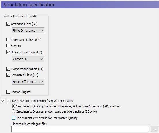
Water Quality¶

In this dialogue, you can also choose to simulate water quality. If you turn on the water quality, then several additional items will be added to the data tree. Also, you will be able to choose to simulate water quality using either the full advection-dispersion method for multiple species including sorption and decay. Or you can choose to simulate water quality using the random walk particle tracking method.

You can also do water quality scenario analysis by using a common water movement simulation and defining only the water quality parameters. The common water movement simulation is defined by first unchecking the Use current WM simulation for Water Quality checkbox.

The Technical Reference contains detailed information on the numerical methods that can be selected from this dialogue:

5. Simulation parameters¶

Once you have selected your processes, then there are several simulation parameters that need to be defined. None of these are initially critical and the default values are generally satisfactory initially. You can come back to all of these at any time.

However, we recommend that you set up you simulation period when you first create your model. The simulation period is used to verify all of you time series data to make sure that your time series cover your simulation period. You can still add your time series files, but if your simulation period is not correct, then you will get a warning message in the message field at the bottom of the page and the time series graphs will not display the proper portion of the time series.

In MIKE SHE, all of the simulation input and output is in terms of real dates, which makes it easy to coordinate the input data (e.g. pumping rates), the simulation results (e.g. calculated heads) and field observations (e.g. measured water levels).

Solver parameters¶

The default solver parameters for each of the processes are normally reasonable and there is usually no reason to change these unless you have a problem with convergence or if the simulation is taking too long to run. For more information on the solver parameters, you should see the individual help sections for the different solvers:

Time step control¶

Likewise, the time step control is important, but the default values are usually reasonable to get your model up and running. Then, you should go back to the Time Step Control dialogue to optimize your simulation time stepping. For more information on time step control, you can see the Controlling the Time Steps section.

Note

Although the different hydrologic processes can run on different time steps, the processes exchange water explicitly. There are restrictions on the relationship between the time steps in the processes. In particular, the longer time steps must be even multiples of the shorter time steps. In other words, a 24-hour groundwater time step can include four 6-hour unsaturated flow time steps, which can each include three 2-hour overland flow time steps. See Time Step Control for more information.

6. Hot starting from a previous simulation¶

Your MIKE SHE simulation can be started from a hot start file. A hot start file is useful for simulations requiring a long warm up period or for generating initial conditions for scenario analysis. Hot starting can also be an effective way to change parameters that are normally static (e.g. hydraulic conductivity) during the model process.

To start a model from a previous model run, you must first save the hot start data, in the Storing of Results dialogue. In this dialogue, you specify the storing interval for hot start data. Then in the Simulation Period dialogue, you can specify the hot start file and then select from the available stored hot start times.

Hot start limitations¶

There are a few limitations and caveats with the hot start process.

MKE 11 and MIKE 1D require an independent hot start.
The Water Quality simulations cannot be started from a hot start file.
There is no append function for the hot start results, so your simulation will generate an independent set of results.
The pre-processed data does not reflect the hot-start information. The pre-processed data is based on the specified input data, not the results file from which the simulation will be started. This primarily affects initial conditions.