Results Tab
1. Overview
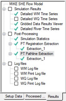
All the simulation results are collected in the Results tab.
The Simulation results are grouped under the Simulation Results section. This includes Detailed time series output for both MIKE SHE and the river, as well as Grid series output for MIKE SHE.
Under the Results Post-processing, you can find tools for extracting and manipulating the simulation results. This is where you will find the tools for extracting the shape file outputs for the Random walk particle tracking simulation. A Simulation Statistics tool is also available for helping you assimilate the calibration statistics for each of the detailed time series plots.
2. Results of Simulation
The Results section includes the direct visualization and analysis of the simulation results
a. MIKE SHE Detailed Time Series
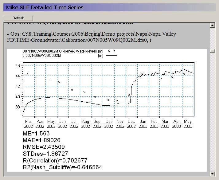
The MIKE SHE Detailed time series tab includes an HTML plot of each point selected in the Detailed WM time series output dialogue. The HTML plots are updated during the simulation whenever you enter the plot, or click on the Refresh button.
When you have more than five detailed time series items, the plots are divided into seperate pages. In this case the main page is a list of the links to the individual plots and each html page includes five plots.
b. Gridded Data Results Viewer
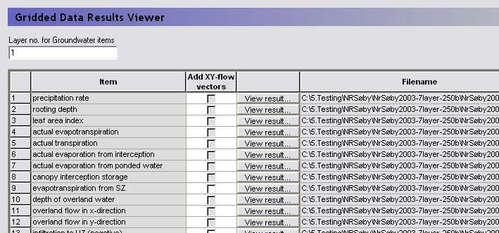
This table is a list of all gridded data saved during a MIKE SHE simulation. The items in the list originate from the list of items selected in the Grid series output dialogue from the Setup tab.
View Result... - Clicking on the View result button will open the Results Viewer to the current item. All overlays from MIKE SHE (e.g. shape files, images, and grid files) will be transferred as overlays to the result view. However, the river network is not transferred as an overlay.
Layer number for Groundwater Items - For 3D SZ data files, the layer number can be specified at the top of the table. However, the layer number can also be changed from within the Results Viewer. By default the top layer is displayed.
Add XY-flow Vectors - Vectors can be added to the SZ plots of results, by checking the Add X-Y flow vectors checkbox. These vectors are calculated based on the Groundwater flow in X-direction and Groundwater flow in Y-direction data types if they were saved during the simulation. In the current version, velocity vectors cannot be added for overland flow output.
file name - The file name column shows the name of the result file from which the gridded data will be extracted.
“The Result Viewer setup file already exists” warning When the Result Viewer opens one of the items in the table, it creates a setup file for the particular view with the extension .rev. The name of the current setup file is displayed in the title bar of the dialogue. Initially, the .rev file includes only the default view settings and the overlay information from MIKE SHE. However, if you make changes to the view, such as changes the way contours are displayed, then when you close the view, you will be asked if you want to save your changes. The next time you open the item in the table, you will be asked if you want to overwrite the existing .rev file. If you click on “Yes”, then a new .rev file will be created with the default values. If you click on “No”, then your previous settings will be re-loaded. This is a convenient way to set up the contouring, legend, etc., the way you want and then re-use the settings. The .rev file can also be loaded directly in the Results Viewer by double clicking on the .rev file or loading the file into the MIKE Zero project explorer.
c. Detailed River Time Series
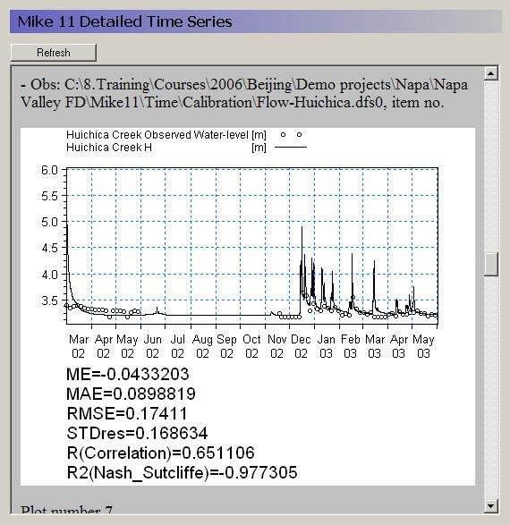
The detailed river time series page includes an HTML plot of each point selected in the Detailed River Time Series Output dialogue. The HTML plots are updated during the simulation whenever you enter the view. Alternatively, you can click on the Refresh button to refresh the plot.
Note that the HTML plot is regenerated every time you enter the view. So, if you have a lot of plots and a long simulation, then the regeneration can take a long time.
When you have more than five detailed time series items, the plots are divided into seperate pages. In this case the main page is a list of the links to the individual plots and each html page includes five plots.
d. Related Items:
- Detailed River Time Series Output
- Statistic Calculations
- Detailed WM time series output
- Statistic Calculations
- Grid series output
- The Results Viewer
3. Results Post-processing
The post-processing section includes options for extracting the results from the various results files.
a. Run Statistics
User interface
Run statistics is a summary of the run statistics for the river model and MIKE SHE detailed time series. The statistics are generated in HTML and shape file format. The calculations include all the detailed time series items that have observation data.
To calculate Run Statistics for a simulation, select the period you want to summarize, then click on the Generate Statistics button. For some simulations with long simulation periods and/or a lot of calibration data it can take several minutes to generate the run statistics.
The Run Statistics are displayed in HTML format on the Run Statistics page (see below).The HTML table can be copied and pasted directly into Microsoft Word or Excel.
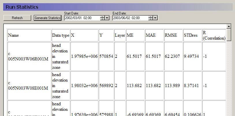
Similar to the detailed time series output, the Run Statistics can be viewed during a simulation. Press the Refresh button on the Run Statistics page to update the Run Statistics using the most recent model results during a simulation
Shape file output for run statistics
A shape file of statistics is also generated when the HTML document is generated. The shape file contains all of the information contained in the HTML document and can be used to generate maps of model errors that can be used to evaluate spatial bias. The shape file is created in the simulation directory and is named projectname_Stat.shp where SimulationName is the name of the *.she file for the simulation. Note: the Run Statistics shape file does not have a projection file associated with it. This file must be created using standard ArcGIS methods.
Statistic Calculations
The statistics contained in the HTML document and the shape file are calculated using the same methods used to calculate statistics for the detailed time series output.
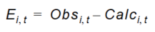
The standard calibration statistics calculated based on the differences between the measured observations and the calculated values at the same location and time. Thus, the error, or residual, for an calculation - observation pair is
Equation 14.01
where
- \(Ei,t\) is the difference between the observed and calculated values at location i and time t.
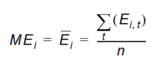
Mean (ME)
The mean error at location i where n observations exist is
Equation 14.02
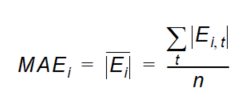
Mean Absolute Error (MAE)
The mean of the absolute errors at location i where n observations exist is
Equation 14.03
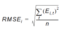
Root Mean Square Error (RMSE)
The root mean square error at location i where n observations exist is
Equation 14.04
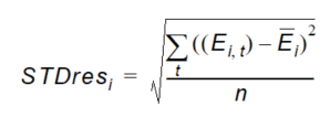
Standard Deviation of the Residuals (STDres)
The standard deviation of the residuals at location i where n observations exist is
Equation 14.05
The standard deviation is a good measure to evaluate how well the dynamics of a certain observation are simulated.
Correlation Coefficient (R)
The correlation coefficient is a measure of the linear dependency between simulated and measured values. The closer the value is to 1.0, the better the match. The correlation coefficient at location i is
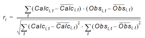
Equation 14.06
where
- \(\bar{Obs}_i\) and \(\bar{Calc}_i\) are the means of the observations and calculations at location i respectively.
Nash Sutcliffe Correlation Coefficient (R2)
The Nash-Sutcliffe coefficient at location i where n observations exist is
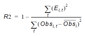
Equation 14.07
where
- \(\bar{Obs}_i\) is the mean of the observations at location i. R2 will be 1.0 if there is a perfect match.
b. Water Balances
It's possible to add Water Balance results to the Results tab. New water balances can be added by clicking on the Insert icon in the Water Balance entry under Post-Processing. The following fields are available for each water balance.
- Enable: If this check box is ticked, then the water balance will be re-computed at the end of each simulate run.
- Name: Optional name field. If blank, the name of the water balance file will be used.
- Water balance configuration file: Path to the water balance file. The Water Balance application can also be opened from here using the Edit button.
After adding a new water balance file, the name is displayed under Water Balance in the Results tab. Individual water balance results are displayed under the water balance name. Individual results are displayed in the same way as in the Water Balance application, and results are updated after each simulation run (if the Enable check box is ticked).
c. PT Registration Extraction
The SZ random walk particle tracking module is very useful for finding out the source of water to an area of interest, for example a well field or a wetland. A property of each particle is its starting location. If the particle is removed from the model or enters a specified area, then the particle is tagged, or ‘registered’. At the end of the simulation, you can then sift through all of the particles and find the starting location for all the ones that you want. With this information, you can build up a dyanamic picture of the source of water entering an area or leaving the model through a specific boundary. The extraction itself will compile a point shape file with the starting locations of all the particles satisfying the specified criteria.
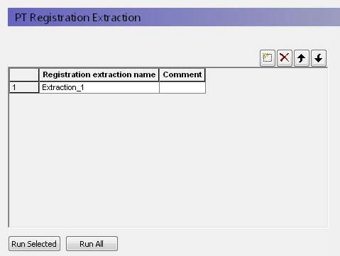
In the top level of this data tree item, you can specify any number of different particle extractions. These will be saved from simulation to simulation, allowing you to re-run the extraction for different scenarios.
The buttons at the bottom, allow you to run the selected extraction or all of the specfied extractions.
Extraction properties
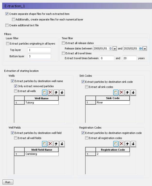
The PT module can generate thousands of particles during a simulation. The extraction definition allows you to specify the criteria finding just the particles that you are interested in.
Create separate shape files for each extracted item - If this option is selected, then you will get a seperate shape file for Wells, Well Fields, Sink Codes and Registration codes.
Additionally, create separate files for each extracted layer - If you have selected the option above, then you also have the option to divide the shape files into one for each numerical layer.
Create additional text file - If this option is selected, a space delimited txt file is created with the fields:
ID / XBirth(meter) / YBirth(meter) / ZBirth(meter / IXBirth / IYBirth / Laye- rBirth / XReg(meter) / YReg(meter) / ZReg(meter) / IXReg / IYReg / LayerReg / BirthTime(year) / TravelTime(year / RegZoneCode / Sink- Code / WellName / WellFieldName.
Filters
For each extraction, the search for relevant particles can be restricted to specific layers and time periods.
Extraction of particle starting locations
The extraction process finds the starting location of all particles that were registered based on the criteria you specify. By default, all the extraction options are turned off. When you active an extraction criteria, by default all particles that meet the criteria will be extracted. For example, particles for all of the sink codes will be extracted. Each different sink code will have a seperate attribute in the shape file. If you want to refine the search criteria, you can optionally specify the criteria in the table.
Note
An individual particle can be registered multiple times. For example, it might pass through a registration zone, then a well cell without being extracted, and then discharge into a river.
Wells - By default, all particles removed by a well are registered. However, particles that enter a cell containing a well are also registered, even if they are not actually removed by the well. For example, they could flow through the cell or not make it to the well before the simulation ends. There is an option in this section to separate out just the particles that were actually removed by the well. The table allows you to specify individual well names as specified in the Well editor.
Well Fields - Each well in the Well Editor can be optionally assigned to a Well Field in the Well Locations table. Using the Well Field option, you can group wells together and calculate the influence area of a the entire group of wells.
Sink Codes - Particles can be removed by various sinks. The sinks can be water sinks, such as a river, or they can be concentration sinks.
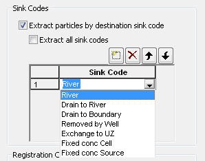
Drain to River/Boundary - Drain sinks refer to saturated zone drainage and are separated by the discharge point, that is SZ drainage flowing to a river or SZ drainage flowing to a boundary node.
Removed by Well - The particle is removed by a well. Note that, particles that may pass through a cell containing a well.
Exchange to UZ - This refers to particles that are removed by capillary flow from SZ into the UZ, or particles that become trapped in the UZ when the water table falls. However, a particle may become trapped and then later reactivated when the water table rises. Each time it is trapped it will be re-registered.
Fixed Conc Cell/Source - Fixed concentration is less than the incoming concentration. Note that the concentration is determined by the particle mass defined in the Particle Tracking Specification dialog.
Registration Codes - The registration codes are user defined zones that create a particle registration whenever a particle passes into the zone. A particle can be registered multiple times, if it passes in and out of the zone. The registration zones are defined in the PT Registration Codes/Lenses dialog. There is no cross-referencing to the list of Registration Codes defined in the simulation, so you have to be careful to specify the code that you want.
d. PT Pathline Extraction
It is too cumbersome to extract and plot the pathlines for all of the thousands of particles that can be generated during a PT simulation. The PT Pathline Extraction utility allows you to extract the pathlines for specific particles if you have saved the intermediate locations in the Storing of Results dialog.
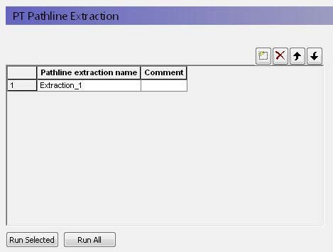
In the top level of this data tree item, you can specify any number of different pathline extractions. These will be saved from simulation to simulation, allowing you to re-run the extraction for different scenarios.
The buttons at the bottom, allow you to run the selected extraction or all of the specified extractions.
Extraction Properties
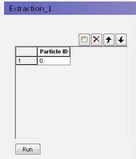
To extract a particle pathline you need a Particle ID. These can only be found after the simulation by evaluating the PT output. For example, you can find the particle ID by extracting the particle start locations that end in a specific well and then finding the ID numbers of the particles that you want in the shape file that was created.
Keep in mind that the PT Pathline Extraction text output is of 'fixed width' type. This output may then be opened in 3rd party software for further processing and analysis.
3. Log Files
The log files section contains a view of two log files per engine. The "WM Log File" and (if included) the "WQ Log File" contain messages, warnings and errors from the WM and the WQ engines. These are the files created in the same folder as the .she file. They are also displayed in the simulation tab when running the engine. The "WM print log file" and the "WQ print log file" contain additional details. They are created in the results directory.