Linear Reservoir Method
The linear reservoir module for the saturated zone in MIKE SHE was developed to provide an alternative to the physically based, fully distributed model approach. In many cases, the complexity of a natural catchment area poses a problem with respect to data availability, parameter estimation and computational requirements. In developing countries, in particular, very limited information on catchment characteristics is available. Satellite data may increasingly provide surface data estimates for vegetation cover, soil moisture, snow cover and evaporation in a catchment. However, subsurface information is generally very sparse. In many cases, subsurface flow can be described satisfactorily by a lumped conceptual approach such as the linear reservoir method.
The MIKE SHE modelling system used with the linear reservoir module for the saturated zone may be viewed as a compromise between limitations on data availability, the complexity of hydrological response at the catchment scale, and the advantages of model simplicity. The combined lumped/physically distributed model was primarily developed to provide a reliable, efficient instrument in the following fields of application:
- Assessment of water balance and simulation of runoff for ungauged catchments
- Prediction of hydrological effects of land use changes
- Flood prediction
The following sections first provide an overview of the linear reservoir theory, followed by detailed descriptions of the implementation in MIKE SHE.
Restrictions
The Linear Reservoir Method is a lumped, conceptual approach and does not support all features available with the 3D Finite Difference Method. In particular, the following are not supported:
- Coupling of the saturated zone to a sewer/collection-system model.
1. Linear Reservoir Theory
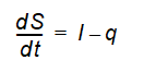
A linear reservoir is one, whose storage is linearly related to the output by a storage constant with the dimension time, also called a time constant, as follows:

Equation 33.30
where - S is storage in the reservoir with dimensions length - k is the time constant - q is the outflow from the reservoir with dimensions length/time.
The concept of a linear reservoir was first introduced by Zoch (1934,1936,1937) in an analysis of the rainfall and runoff relationship. Also, a single linear reservoir is a special case of the Muskingum model, Chow (1988).
a. A Single Linear Reservoir with One Outlet
The continuity equation for a single, linear reservoir with one outlet can be written as
Equation 33.31
where - t is time - I is the inflow to the reservoir
Combining equation (33.8)) and (33.9) yields a first-order, linear differential equation which can be solved explicitly
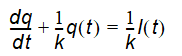
Equation 33.32
(I) to the reservoir is assumed constant, the outflow (q) at the end of a time step dt can be calculated by the following expression
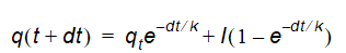
Equation 33.33
a. A Single Linear Reservoir with Two Outlets
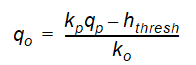
The outflows from a linear reservoir with two outlets can also be calculated explicitly. In this case storage is merely, instead of Eq. (1) given as
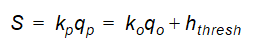
Equation 33.34
where - kP is the time constant for the percolation outlet, - qp is percolation, - ko is the time constant for the overflow outlet, - qo is outflow from the overflow outlet, and - hthresh is the threshold value for the overflow outlet.
Combining equation (33.34) and (33.32) and solving for S, still assuming I is constant in time, yields the following expressions for qp and qo at time (t+dt).
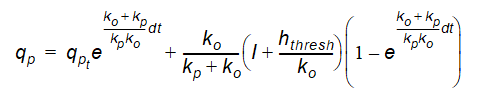
Equation 33.35
Equation 33.36
2. General Description
In the linear reservoir method, the entire catchment is subdivided into a number of subcatchments and within each subcatchment the saturated zone is represented by a series of interdependent, shallow interflow reservoirs, plus a number of separate, deep groundwater reservoirs that contribute to stream baseflow. An example of a subdivision of a catchment area is outlined in Figure 33.8, where the topographical zones represent the interflow reservoirs in the model. If a river is present, water will be routed through the linear reservoirs as interflow and baseflow and subsequently added as lateral flow to the river. If no river is specified, the interflow and baseflow will be simply summed up and given as total outflow from the catchment area. The lateral flows to the river (i.e. interflow and baseflow) are by default routed to the river links that neighbour the model cells in the lowest topographical zone in each subcatchment.
Interflow will be added as lateral flow to river links located in the lowest interflow storage in each catchment. Similarly, baseflow is added to river links located within the baseflow storage area.
The infiltrating water from the unsaturated zone may either contribute to the baseflow or move laterally as interflow towards the stream. Hence, the interflow reservoirs have two outlets, one outlet contributes to the next interflow reservoir or the river and the other contributes to the baseflow reservoirs. The baseflow reservoirs, which only have one outlet, are not interconnected.
Normally, one reservoir should be sufficient for modelling baseflow satisfactorily. However, in some cases, for example in a large catchment, hydraulic contact with a river is unlikely to be present everywhere. In this case, more than one reservoir can be specified.
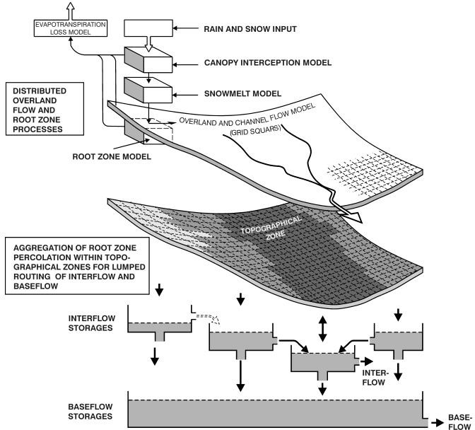
Figure 33.7 Model Structure for MIKE SHE with the linear reservoir module for the saturated zone
In low areas adjacent to the river branches the water table may, in periods, be located above or immediately below the surface. In this case, it will contribute more to total catchment evaporation than the rest of the area. To strengthen this mechanism water held in the part of the baseflow reservoirs beneath the lowest interflow zone may be allowed to contribute to the root zone when the soil moisture is below field capacity.
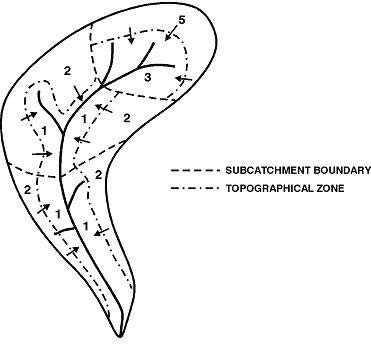
Figure 33.8 Example of Desegregation of a Catchment into Sub-catchments and Topographical Zones
Previous experience with lumped conceptual models shows that the linear reservoir approach is sufficient for an accurate simulation of the interflow and baseflow components, if the input to the reservoirs can be assessed correctly and the time constants of the outlets are known. Due to the distributed approach and physically based representation used in MIKE SHE in the overland and unsaturated zone flow components, an accurate simulation of soil moisture drainage in space and time is provided in MIKE SHE for the linear reservoir module. The time constants on the other hand are basically unknown for an ungauged catchment but a fair estimate may be obtained from an evaluation of the hydrogeologic conditions and/or from gauged catchment with similar subsurface conditions.
If the UZ feedback is not included, uncertainty of the time constants will only affect routing of the baseflow and interflow components while the total volumes of runoff will remain unchanged. If UZ feedback from the baseflow reservoir is included, some of the baseflow to the stream will be transferred to the UZ storage because of ET in the unsaturated zone.
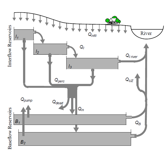
Figure 33.9 Schematic flow diagram for the Subcatchment-based, linear reservoir flow module
3. Subcatchments and Linear Reservoirs
Three Integer Grid Code maps are required for setting up the framework for the reservoirs,
- a map with the division of the model area into Subcatchments,
- a map of Interflow Reservoirs, and
- a map of Baseflow Reservoirs.
The Interflow Reservoirs are equivalent to what was called the Topographic Zones in earlier versions of the Linear Reservoir module in MIKE SHE. There is no limit on the number of subcatchments, or linear reservoirs that can be specified in the model.
The division of the model area into subcatchments can be made arbitrarily. However, the Interflow Reservoirs must be numbered in a more restricted manner. Within each subcatchment, all water flows from the reservoir with the highest grid code number to the reservoir with the next lower grid code number, until the reservoir with the lowest grid code number within the subcatchment is reached. The reservoir with the lowest grid code number will then drain to the river links located in the reservoir. If no river links are found in the reservoir, then the water will not drain to the river and a warning will be written to the run log file. For example, in Figure 33.8. Interflow Reservoir 2 always flows into Reservoir 1 and Reservoir 1 discharges to the stream network. Likewise, Reservoir 5 flows into 3, which discharges to the stream network.
For baseflow, the model area is subdivided into one or more Baseflow Reservoirs, which are not interconnected. However, each Baseflow Reservoir is further subdivided into two parallel reservoirs. The parallel reservoirs can be used to differentiate between fast and slow components of baseflow discharge and storage.
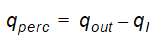
Figure 33.9 is a schematization of the flow to, from and within the system of linear reservoirs. Vertical infiltration from the unsaturated zone is distributed to the Interflow Reservoirs (Qinfil). Water flows between the Interflow Reservoirs sequentially (QI) and eventually discharges directly to the river network (QI river), or percolates vertically to the deeper Baseflow Reservoirs (Qperc). The parallel Baseflow Reservoirs each receive a fraction of the percolation water (Qin) and each discharges directly to the river network (QB). Groundwater can be removed from the Baseflow Reservoirs via groundwater pumping (Qpump). If UZ feedback is included, then some of the baseflow to the stream will be added to the UZ storage (QUZ) and subsequently removed from the unsaturated zone via ET.
In some situations, the interflow reservoirs will not correspond to the areas of active baseflow in the current catchment. That is, some percolation from the interflow reservoirs may contribute to baseflow in a neighbouring watershed. This has been resolved by introducing a dead zone storage (Qdead) between the Interflow and Baseflow Reservoirs
4. Calculation of Interflow
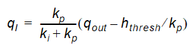
Each Interflow Reservoir is treated as A Single Linear Reservoir with Two Outlets. Thus, from Eq. 33.30, if the water level in the linear reservoir is above the threshold water level
Equation 33.37
where - qI is the specific interflow out of the reservoir in units of [L/T], - h is the depth of water in the interflow reservoir, - hthresh is the depth of water required before interflow occurs, - ki is the time constant for interflow. If the water level is below the threshold there is no interflow.
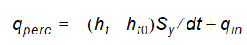
Similarly, if there is water in the linear reservoir, specific percolation outflow can be calculated from
Equation 33.38
where h is again the depth of water in the interflow reservoir, kp is the time constant for percolation flow. If the water level is at the bottom of the reservoir there is no percolation.
Combining Eqs 33.37 and 33.38 with the continuity equation
Equation 33.39
where: - qin is the sum of inflow from an upstream Interflow reservoir and the infiltration from UZ, - Sy is the specific yield, gives the following expression for h at time t when there is both qI and qperc (linear reservoir with two outlets)
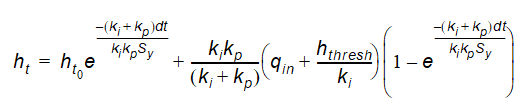
Equation 33.40
In the case where the water level is below the threshold, the formulation for a linear reservoir with one outlet applies, which yields
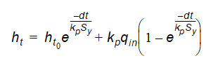
Equation 33.41
Inflow to the Interflow reservoir, qin, will normally be positive (i.e. water will be being added), but if evapotranspiration from the saturated zone is included or the net precipitation is used as input there might be a net discharge of water from the interflow reservoir. As the infiltration is a constant rate calculated explicitly in other parts of MIKE SHE, this will result in a water balance error if the interflow reservoir is empty. This will be reported in the log file at the end of the simulation.
From the level changes in the reservoir, the total average outflow can be calculated for the time step, dt. Thus, for the two outlet case,
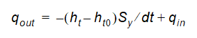
Equation 33.42
Equation 33.43
Equation 33.44
and for the single outlet case (no interflow),
Equation 33.45
If during a time step the reservoir level crosses one or more thresholds, an iterative procedure is used to subdivide the time step and the appropriate formulation is used for each sub-time step.
The discharge to the river, qI river, in the lowest Interflow Reservoir is simply the qI from that reservoir.
5. Calculation of Interflow Percolation and Dead Zone Storage
The inflow to the Baseflow Reservoirs from the Interflow Reservoirs, qv, is weighted based on the overlapping areas. Thus, if the Baseflow and Interflow reservoirs overlap, then
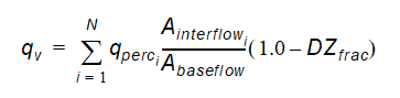
Equation 33.46
where - Ainterflow is the area of the Interflow Reservoir that overlaps with the Baseflow Reservoir, - Abaseflow is the area of the Baseflow Reservoir - DZfrac is the fraction of the total Qin that goes to the dead zone storage.
Likewise, the amount of water going to deadzone storage is given by
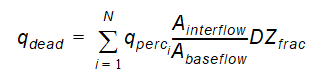
Equation 33.47
6. Calculation of Baseflow
From Eq. 33.30, if the water level in the linear reservoir is above the threshold water level
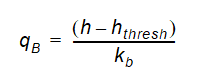
Equation 33.48
where - h is the depth of water in the baseflow reservoir, - hthresh is the depth of water required before baseflow occurs, - kb is the time constant for baseflow. If the water level is below the threshold there is no baseflow.
Similar to Eq. 33.39, for each Baseflow Reservoir
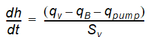
Equation 33.49
where - qIN is the amount of inflow to each base flow reservoir, - qB is the specific baseflow out of the reservoir, - qpump is the amount of water removed via extraction wells from each reservoir. Both qv and qpump are controlled by split fractions that distribute qv and qpump between the two parallel baseflow reservoirs.
Each Baseflow Reservoir can be treated as A Single Linear Reservoir with One Outlet. Thus, as long as the water level is above the threshold water level for the reservoir (i.e. there is still baseflow out of the reservoir),
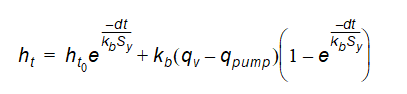
Equation 33.50
where - kb is the time constant for the Baseflow Reservoir.
The formula for a single outlet is applicable because there is no time constant associated with the pumping. However, Qpump, is also controlled by a threshold level, in this case, a minimum level below which the pump is turned off. Since this minimum level is independent of the threshold level for the reservoir itself, a case could arise, whereby there was pumping, but no baseflow from the reservoir. In this case,
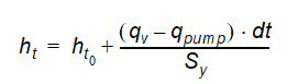
Equation 33.51
If there is no pumping and no baseflow out, then the expression for the water level in the reservoir simply becomes
Equation 33.52
In general, during a time step, the water level may cross one or more of the pumping or the baseflow thresholds. If this occurs, the program uses an iterative procedure to split the time step into sub-time steps and applies the appropriate formulation to each sub-time step.
7. UZ Feedback
A feedback mechanism to the unsaturated zone has been included in the module to model a redistribution of water in favour of evapotranspiration from the low wetland areas located adjacent to most rivers.
The UZ feedback is not relevant if the Richards Equation method is used and the feedback fraction should be set to zero.
Water is redistributed from the base flow reservoirs to the unsaturated zone model in the lowest interflow reservoir zone of the subcatchment, if there is a water deficit in the root zone. The base flow discharge is distributed to all UZ columns in the lowest interflow reservoir.
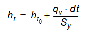
The UZ deficit in the lowest interflow reservoir is called the Field Moisture Deficit (FMD) in units of metres, and is calculated as the total amount of water required to bring the entire root zone in all the UZ columns back up to field capacity. Thus,
Equation 33.53
where - \(\theta_{FC}\) is the moisture content at field capacity, - \(\theta\) is the moisture content in the root zone, - n is the number of UZ cells in the root zone, - \(\Delta_z\) is the height of the UZ cell.
This is then summed over all of the UZ columns in the lowest interflow reservoir.
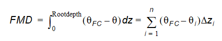
Now, the amount of water that is available from the linear reservoirs to be redistributed to the unsaturated zone is calculated as a fraction of the baseflow:
Equation 33.54
where - UZfrac is a specified fraction of the baseflow that is allowed to recharge the unsaturated zone.
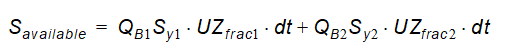
If Savailable is larger than or equal to the Field Moisture Deficit, then the water content of each of the root zone cells is increased to field capacity.
If Savailable is smaller than the Field Moisture Deficit, then the water content of each of the root zone cells is proportionally increased by
Equation 33.55
After the feedback calculation, the amount of baseflow to the river is reduced by the amount of water used to satisfy the Field Moisture Deficit in the unsaturated root zone, which is QUZ, in Figure 33.9.
8. Coupling to Rivers
The discharge from the lowest Interflow Reservoir in each subcatchment is distributed evenly over the river model nodes located in the reservoir. Like- wise, the baseflow from the Baseflow Reservoirs is distributed over the same nodes. The default distribution can be overridden by specifying specific river branches and chainages.
If the river branch is defined as a “losing branch” then water will be added to the baseflow reservoir based on the head in the river, the river width and the riverbed conductivity specified.
Note
The lowest linear reservoir discharges to the river network. However, if the lowest linear reservoir is not connected to a river branch, then the linear reservoir will still discharge. The only difference is that no water will be added to the river. This situation can arise when there are no river branches in small subcatchments. A warning will be written to the log file if a subcatchment is not connected to a river branch.
9. Limitations of the Linear Reservoir Method
The Linear Reservoir method is a simple method for calculating overall water balances in the saturated zone. As such, it is unsuitable when a detailed spatial distribution of the water table is required. However, even given the simplicity of the method, the following simplifications and limitations should be noted:
- In the Linear Reservoir Method, the same river links are used for both of the base flow reservoirs. This is a limitation in the sense that occasionally you may find that fast response and the slow response baseflow may contribute to different parts of the stream.
- When calculating the unsaturated flow, the bottom boundary condition is input from a separate file - not calculated during the simulation. This means that changes in the water levels in the reservoirs will have no effect on the UZ boundary condition.
- The numerical solution used for the Linear Reservoir module assumes that the inflow to each of the linear reservoirs is constant within a time step. Strictly speaking, this is not correct as outflow from each reservoir changes exponentially during a time step. The calculation procedure uses the mean outflow from the upper reservoir as inflow to the downstream reservoir. In this way, there is no water balance error but the dynamics are somewhat dampened. If this is a problem, smaller time steps can be chosen, which will lead to a more accurate solution, as the changes in flow become smaller during each time step.