Advection Dispersion

1. Simulation control

In the MIKE SHE water quality module, you can calculate solute transport in the different parts of the hydrological cycle. In the present version of MIKE SHE AD only three combinations are legal:

• groundwater transport can run as a stand-alone module,
• groundwater transport can be run in combination with the overland transport module, and
• all modules in combination can run.

Thus, a simulation with only overland or only the unsaturated zone is not possible and that combinations of the unsaturated zone with only the overland or groundwater component are not possible.

a. Flow Storing Requirements

The transport calculations are based on the water flow, water contents, hydraulic heads and water levels calculated in a MIKE SHE water movement simulation. Depending on the complexity of the advection/dispersion simulation, the water movement output must be stored with different storing time steps. The selected storing frequency should be sufficient to reflect the dynamics of the flow processes. However, the following two restrictions must be observed:

• The SZ head and SZ flow storing time steps must be equal, and
• The SZ storing time step must be an integer multiple of the UZ storing time step, which must be an integer multiple of the overland storing time step.

The last restriction above is controlled in the user interface.

b. Internal Boundary Conditions

If a simulation with MIKE SHE AD includes more than one part of the hydrological cycle, the solute fluxes between the different hydrologic components must be kept track of. In principle, the solute fluxes between the components follow the water flow between the components. Multiplying the flow rate with the solute concentration produces a source/sink term for the relevant components. Table 36.1 lists the solute exchange possibilities between the components, in particular when one or more component is not included in the flow simulation.

Table 36.1 Internal boundary source/sinks between hydrologic components in MIKE SHE AD

Solutes from:	Primary solute sink:	Alternative solute sink (if primary sink unavailable):
Precipitation Fluxes	Overland flow	Unsaturated zone or Groundwater
Overland Fluxes Infiltration Overland flow	Unsaturated zone River	Groundwater External boundary (none)
Unsaturated Zone Fluxes Infiltration Bypass flow	Groundwater	External Boundary
Groundwater Fluxes SZ Drainage Upward flux to overland Upward flux to UZ Baseflow to streams	Overland flow Unsaturated Zone River	Overland flow or External boundary (none) Overland flow (none)
River Baseflow to groundwater	Groundwater	(none)

An sketch of the different internal boundary conditions is shown in Figure 36.1. Each of these exchanges is detailed in the respective sub-section for each hydrologic component.

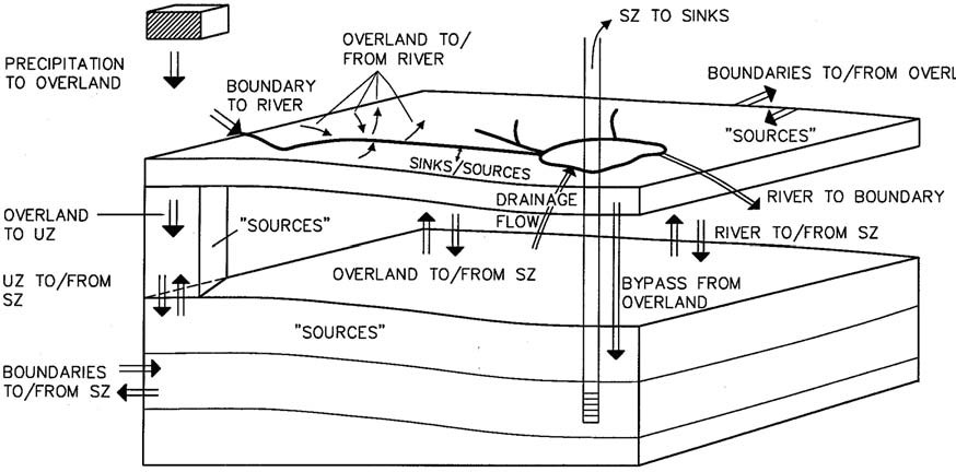
Figure 36.1 Outline of the different transport possibilities between components and boundaries.

c. Time step calculations

The time scales of the various transport processes are different. For example, the transport of solutes in a river is much faster than transport in the groundwater. The optimal time step is different for each component, where ‘optimal’ can be defined as the largest possible time step without introducing numerical errors. In addition, the optimal time step varies in time as a consequence of changing conditions in the hydrological regime within the catchment.

Different time steps are allowed for the different components. However, an explicit solution method is used, which sometimes requires very small time steps to avoid numerical errors. The Courant and Peclet numbers play an important role in the determination of the optimal time step.

The user can specify the maximum time step in each of the components. However, the actual simulation time step is controlled by the stability criterions, with respect to advective and dispersive transport, as well as the timing of the sources and sinks, and the simulation and storing time steps in the WM simulation.

In Figure 36.2, you can see an example of the sequence of calling each components in the MIKE SHE advection-dispersion module. The time step in the river transport calculation is usually the smallest, whereas time step for groundwater transport is always the largest.

A transport simulation begins with the overland component followed by the river model, the unsaturated zone component and the groundwater component. Figure 36.2 shows how the simulation time steps can be controlled solely by the storing time step in the flow simulation.

Solute sources and the storing of data in the different components influences the time step. For example, in Figure 36.2, a SZ source requires that all components have a break when the source starts.

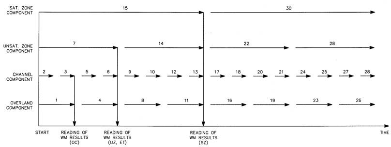
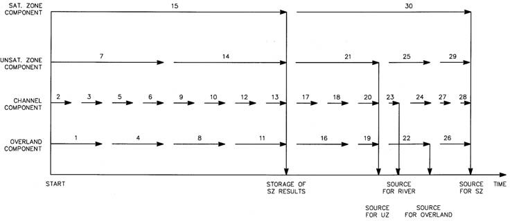
Figure 36.2 An example calculation sequence for solute transport in MIKE SHE.

Time step limitations

For each component the maximum allowable time step is determined by the advective and dispersive Courant number.

The advective Courant number in the x-direction, \(\sigma x\), is defined as:

Equation 36.01

and the dispersive Courant number,\(\Gamma x\), is defined as:

Equation 36.02

The limitations are different in each flow component and will be described in more detail under the respective flow component sections.

You can also specify a maximum time step for each component, as well as a limiting solute flux per time step.

2. Solute Transport in the Saturated Zone

The solute transport module for the saturated zone in MIKE SHE allows you to calculate transport in 3D, 2D, layer 2D, or even 1D. However, the transport formulation is controlled by the water movement discretisation. If the vertical discretisation is uniform (except for the top and bottom layer) the transport scheme is described in a fully three-dimensional numerical formulation. If the numerical layers have different thicknesses a multi-layered 2D approach is used, where each layer exchanges flows with other layers as sources and sinks. If you specify a 1D or 2D flow simulation, the transport formulation is further simplified.

Temporal and spatial variations of the solute concentration in the soil matrix are described mathematically by the advection-dispersion equation and solved numerically by an explicit, third-order accurate solution scheme.

The forcing function for advective transport is the cell-by-cell groundwater flow, as well as groundwater head, boundary, drain and exchange flows, which are all read from the WM results files. Solute exchange between the other hydrologic components is generally simulated by means of explicit sources and sinks.

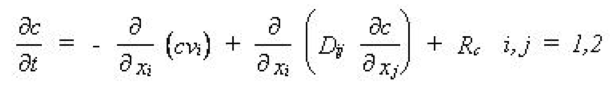
a. Governing Equations

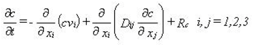
The transport of solutes in the saturated zone is governed by the advection-dispersion equation, which for a porous medium with uniform porosity is

Equation 36.03

where

• \(c\) is the concentration of the solute
• \(R_c\) is the sum of the sources and sinks
• \(D_{ij}\) is the dispersion coefficient tensor
• \(v_i\) is the velocity tensor

The advective transport is determined by the water fluxes (Darcy velocities) calculated during a MIKE SHE WM simulation. To determine the groundwater velocity, the Darcy velocity is divided by the effective porosity

Equation 36.04

where

• \(q_i\) is the Darcy velocity vector
• \(\theta\) is the effective porosity of the medium

The mathematical formulation of the dispersion of the solutes follows the traditional formulations generalised to three dimensions. This formula was developed assuming that the dispersion coefficient is a linear function of the mean velocity of the solutes. In the three-dimensional case of arbitrary flow- direction in an anisotropic aquifer, the dispersion tensor, Dij, contains nine elements, giving a total of 36 dispersivities. The general formulation of the dispersion tensor is

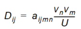
Equation 36.05

where

• \(a_{ijmn}\) is the dispersivity of the porous medium (a fourth order tensor)
• \(v_n\) and \(vm\) are the velocity components
• \(U\) is the magnitude of the velocity vector

The derivation of \(D_{ij}\) and \(a_{ijm}\) in MIKE SHE follows the work of Bear and Verruijt (1987). Two simplifications have been introduced with respect to dispersivity

• isotropy, and
• anisotropy with axial symmetry around the z-axis.

These simplifications are reflected in the number of non-zero dispersivities to be specified. Under isotropic conditions the dispersivity tensor, \(a_{ijmn}\), solely depends on the longitudinal dispersivity, \(\alpha_L\), and the transversal dispersivity, \(\alpha_T\), in the following manner:

Equation 36.06

where

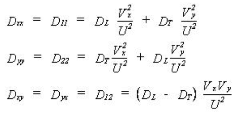
• \(\delta_{ij}\) is the Kronecker delta (with \(\delta_{ij}=0\) for \(i \ne j\) and \(\delta_{ij}=1\) for \(i=j\)). In the Cartesian co-ordinate system applied in MIKE SHE, the velocity components in the coordinate directions are denoted \(V_x\), \(V_y\) and \(V_z\). Thus, we obtain the following expressions for the dispersion coefficients:

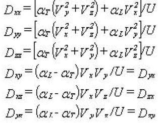
Equation 36.07

This is the general equation for the dispersion coefficients in an isotropic medium for an arbitrary mean flow direction. If the mean flow direction coincides with one of the axis of the Cartesian coordinate system the expression for the dispersion coefficients simplifies even further (e.g. if \(V_y\) and \(V_z\) are equal to zero then \(D_{xy}\), \(D_{xz}\) and \(D_{yz}\) will also be zero).

Under fully anisotropic conditions, the dispersion coefficients depend on 36 dispersivities which is impractical to handle and estimate in practice. Thus, if we assume that the porous medium is symmetric around one of the axis, the number of non-zero dispersivities can be limited to five. This assumption is true if the medium is made up of layers normal to the axis of symmetry, which is the case for some geological deposits. Under these conditions the following expression for the \(a_{ijmn}\) terms (Bear and Verruijt (1987)) have been derived:

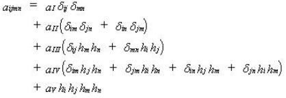
Equation 36.08

where

• \(a_I\), \(a_{II}\), \(a_{III}\), \(a_{IV}\) and \(a_V\) are independent parameters and h is a unit vector directed along the axis of symmetry. In MIKE SHE AD it is assumed that the axis of symmetry always coincides with the z-axis and h becomes equal to (0,0,1).

Five dispersivities are then introduced:

• \(\alpha_{LHH}\) - the longitudinal dispersivity in the horizontal direction for horizontal flow
• \(\alpha_{THH}\) - the transversal dispersivity in the horizontal direction for horizontal flow
• \(\alpha_{LVV}\) - the longitudinal dispersivity in the vertical direction for vertical flow
• \(\alpha_{TVH}\) - the transversal dispersivity in the vertical direction for horizontal flow
• \(\alpha_{THV}\) - the transversal dispersivity in the horizontal direction for vertical flow

Thus, the dispersion coefficients can be written explicitly by combining Eq. (36.5) and Eq. (36.8) as follows:

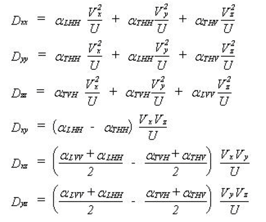
Equation 36.09

and for symmetrical reasons \(D_{xy} = D_{yx}\), \(D_{xz} = D_{zx}\) and \(D_{yz} = D_{zy}\).

Note that Eq. (36.9) can simplify to Eq. (36.7) if \(\alpha_{LHH}=\alpha_{LVV}=\alpha_L\) and \(\alpha_{THH}=\alpha_{TVH}=\alpha_{THV}=\alpha_T\)

Burnett and Frind /11/ suggest that the dispersion should at least allow for the use of two transverse dispersivities - a horizontal transverse dispersivity and a vertical transverse dispersivity - to describe the difference in transverse spreading which is greater in the horizontal plane than in the vertical plane. In comparison, MIKE SHE uses all five dispersivities.

The determination of the five dispersivities is always difficult so often one has to rely on experience or on empirically derived values.

The dispersion term in the advection-dispersion equation accounts for the spreading of solutes that is not accounted for by the simulated mean flow velocities (the advection). Therefore, it is obvious that the more accurate you describe the spatial variability in the hydrogeologic regime and if the grid is sufficiently fine (i.e. the variations in the advective velocity) the smaller the dispersivities you need to apply in the model. Recent laboratory and field research have shown a relationship between the spatial variability of hydrogeologic parameters and the dispersivities. However, it is still difficult to obtain sufficient knowledge about the spatial variability of, for example the hydraulic conductivity, to determine macro dispersivities applicable for solute transport models.

b. Solution Scheme

Regular Grid

The numerical solution to the advection-dispersion equation in MIKE SHE AD is based on the QUICKEST method. Leonard /38/ originally introduced this method, which was further developed by Vested et. al. /53/. It is a fully explicit scheme, which applies upstream differencing for the advection term and central differencing for the dispersion term. The equations are developed to third order and the scheme is mass conservative.

When the vertical discretisation is defined in a regular grid with uniform thickness of all layers except the upper and the lower ones the numerical scheme follows the fully three-dimensional formulation below.

Neglecting the dispersion terms and the source/sink term and assuming that the flow field satisfies the equation of continuity and varies uniformly within a grid cell the advection-dispersion equation may be written in mass conservation form as:

Equation 36.10

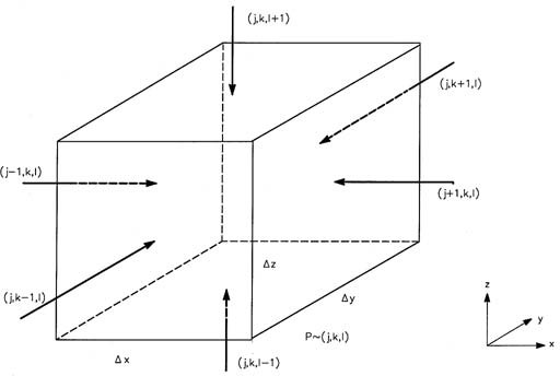
Figure 36.3 Control volume defining an internal SZ grid.

For the control volume shown in Figure 36.3 this equation is written in finite difference form as:

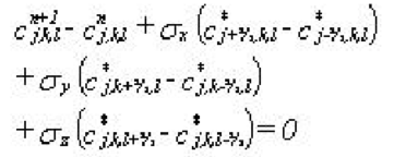
Equation 36.11

where - \(n\) denotes the time index.

In Eq. (36.11) \(\sigma_x\), \(\sigma_y\) and \(\sigma_z\) are the directional Courant numbers defined by

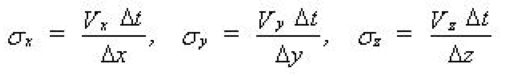
Equation 36.12

and the c-terms are the concentrations at the surface of the control volume at time n*. As these terms are not located at nodal points they have to be interpolated from known concentration values:

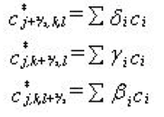
Equation 36.13

The concentration ci is the concentration around the actual point, for example (j-1,k-1,l) and the weights \(\delta_i\), \(\gamma_i\) and \(\beta_i\) are determined in such a way that the scheme becomes third-order accurate. The determination of the weights is demonstrated in Vested et al. (1992) and their values are listed in Table 36.2.

A number of 8 weights has proven to be an adequate choice and their location for the determination of the \(c_{j+½,k,l}\) is shown in Figure 36.4. The other “boundary” concentrations are found in a similar way.

Table 36.2 Weight functions for advective transport

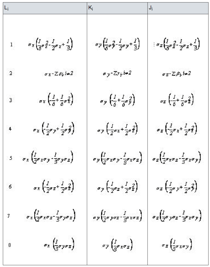
The locations of the weights are determined by the points that enter into the discretisation and because the scheme is upstream centred the weights are positioned relative to the actual direction of the flow.

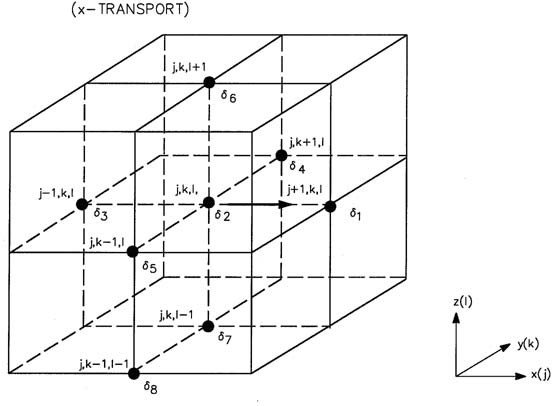
Figure 36.4 Location of interpolation weights for determination of concentrations at the location (j+½,k,l) - a grid boundary.

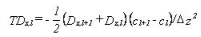
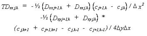
The dispersive transport can be derived in a similar way. With the finite difference formulation of the dispersive transport components based on upstream differencing in concentrations and central differencing in dispersion coefficients the transport in the x-direction can be expressed in the following manner:

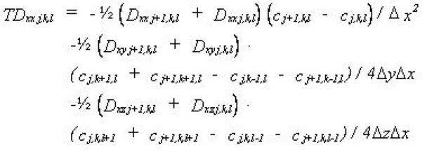
Equation 36.14

The dispersive transports in the other directions are expressed in a similar way. The dispersive transports are incorporated in the weight functions so that the mass transports can be calculated in one step.

Irregular Grid

In general the flow simulation may use varying layer thickness for the vertical discretisation of the saturated zone domain. In this case, the code checks each layer to see whether its thickness is identical with the thickness of the layer above and the layer below in each of the grid cells. If this is the case this layer is handled as described for “regular grid” above (3D). If this is not the case a different approach is followed where a 2D regular grid solution based on the QUICKEST scheme is used for the horizontal transport and the vertical transport is taken into account as an explicit sink/source term.

c. Initial Conditions

The initial concentration is a fully distributed concentration field, which can be entirely uniform or constant by layer.

A boundary water flux into the model, results in a constant concentration boundary at the initial concentration value, unless explicitly specified as a time varying concentration boundary.

d. Source/Sinks, Boundary Conditions and other Exchanges

Boundary conditions for the groundwater transport component can be either

• a prescribed concentration (Dirichlet's condition), or
• prescribed flux concentration (Neumann's condition).

Catchment boundary cells with a specified head are treat as fixed concentration cells with a concentration equal to the initial concentration. A prescribed, time-varying concentration boundary can be specified at any internal node.

Prescribed flux concentration can be specified on the catchment boundary, as well as in any cell inside the model area. The flux concentration at the catchment boundary can be constant or time-varying.

Sinks can either extract pure water (concentration equal to zero) or water with the current concentration. Soil evaporation is the only sink, which removes water with a concentration equal to zero. Sinks where the concentration is equal to the actual solute concentration in the grids include pumping wells, drains and river nodes.

Referring back to Figure 36.1, you should note that

• If UZ transport is included, the upper boundary for the groundwater transport is the exchange of mass with the UZ component. Infiltration from (and to) the unsaturated zone is treated as a source (or sink) term. However, if the UZ flow had a shorter storing time step than the SZ flow, the concentration in the top layer of the SZ transport is updated at the UZ time step.
• If UZ bypass flow was specified, mass is transferred directly from the overland to the groundwater, with the flux equal to bypass flow multiplied with the concentration on the overland.
• Direct exchange between OL flow and SZ flow occurs when the soil is completely saturated. In this case, the infiltration from OL goes directly to the SZ and the mass flux is equal to the infiltration multiplied with the concentration on the overland.
• Exchanges with the river are also treated explicitly as exchange flows. Inflow and outflow respectively are multiplied by the concentration in the river or the adjacent grids to the groundwater.
• SZ Drainage to the overland or the river (or the boundary) is also treated as an SZ sink and the mass receiving component and is again calculated by multiplying the exchange flux with the concentration.

e. Additional options

Disable SZ solute flux to dummy UZ

The following Extra Parameter is useful, if you are using an alternative UZ model, such as DAISY, in MIKE SHE and you are trying to couple it to the WQ.

In this case, you will be typically using the Negative Precipitation option. If you use this option, then you will not use a MIKE SHE UZ, and the UZ-SZ exchange will pass through a “dummy UZ” layer. When this is coupled to the water quality, solutes will also be passed to this dummy UZ layer and removed from the SZ domain and the model.

To prevent the upflow of solutes from SZ to the dummy UZ, you must specify the following Extra Parameter..

Parameter Name	Type	Value
disable sz transport to dummy uz	Boolean	On

SZ boundary dispersion

A detailed test of the MIKE SHE WQ engine comparing an SZ model with fixed concentration at an inflow boundary with an analytical solution for a fixed concentration source, showed that MIKE SHE underestimates the mass flux into the model when the model includes longitudinal dispersion.

The problem is that the SZ transport scheeme (QUICKEST) doesn't include dispersive transport to/from open boundary cells. This is as designed, but apparently not correct. After including the boundary dispersion, the mass input to the model is within 2 % of the analytical solution.

From Release 2011 and onwards, the boundary dispersion has been made optional for backwards compatibility and is activated with the extra-parameter: .

Parameter Name	Type	Value
enable sz boundary dispersion	Boolean	On

However, the SZ boundary dispersion option (above) does not calculate dispersive transport to an inflow boundary correctly. Again, this problem was identified in the tests of MShe_WQ with MIKE ECO Lab vs analytical solution. For example:

• Species 1 enters the model via an inflow (flux) boundary with fixed concentration - including dispersive transport due to the new sz boundary dispersion option.
• Species 1 decays to Species 2 which again decays to Species 3.
• The concentrations of Sp2 & Sp3 are too high, especially close to the inflow boundary.

The analytical solution includes dispersive transport of Sp2 & Sp3 against the flow direction because the concentration of these species are 0 at the boundary. However, this dispersive mass flux to the boundary is not included in the SZ solver due to an old check in the code. When mass flux to/from a boundary point is reversed compared to the flow direction, the mass flux is simply reset to 0.

This made sense before the boundary dispersion was implemented because advective transport against the flow direction would be wrong. But, now, when the boundary dispersion is active, this situation is allowed.

f. Transport in Fractured Media

MIKE SHE AD is able to simulate solute transport in fractured media under some simplifying conditions. If we assume that water flows only in the fractures and that solutes can enter into the soil matrix as immobile solutes the advection-dispersion equation changes to:

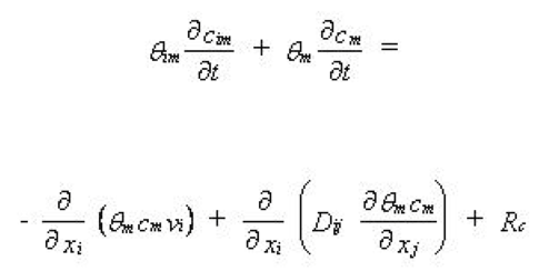
Equation 36.15

where - \(c\) is the concentration of the solute, subscripts m and im are for mobile and immobile, respectively, - \(R_c\) is the sources or sinks - \(D_{ij}\) is the dispersion tensor - \(v_i\) is the velocity tensor determined from fracture porosity.

The exchange of mass between the mobile water phase in the fractures and immobile water phase is described by the traditional diffusion equation:

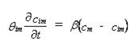
Equation 36.16

where - \(\beta\) is the diffusion coefficient.

Diffusive exchange is included as a distributed source/sink term in the basic advection-dispersion equation.

3. Solute Transport in the Unsaturated Zone

The Solute Transport in the Unsaturated Zone links the transport in the overland flow and transport in the saturated zone together.

Solute transport in the unsaturated zone be simulated in both the soil matrix and macropores. Solute transport in the soil matrix is described by a 1D, unsaturated formulation of the advection-dispersion equation, which is considerably simpler than the 3D formulation in the saturated zone.Although, the unsaturated water movement calculations can be lumped together to save computational time, solute transport in the unsaturated zone is always calculated in every column. The solute transport boundary conditions and initial conditions are specified independent of any column lumping that was done in the water movement simulation.

a. Governing Equations Soil Matrix Transport

For unsaturated solute transport in the soil matrix the advection-dispersion equation is

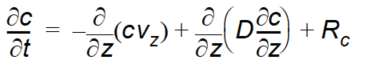
Equation 36.17

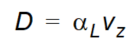
where - \(c\) is the concentration of the solute - \(R_c\) is sum of sources and sinks - \(D\) is the dispersion coefficient - \(v_z\) is the vertical velocity

The advective transport is determined by the water flux calculated during a MIKE SHE WM simulation. As the water flow is assumed strictly vertical, this restriction applies also to the advective transport of the dissolved solutes.

To determine the velocity, vz, the flux is divided by the moisture content:

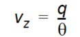
Equation 36.18

The mathematical formulation of the dispersion of the solutes follows the formulation derived for groundwater flow with a linear relation between the dispersion coefficient and the seepage velocity but limited to one dimension. In this case the dispersion coefficient can be written as:

Equation 36.19

where - \(\alpha_L\) is the longitudinal dispersivity of the porous medium which represents the heterogeneity of the soil hydraulic parameters. \(\alpha_L\) is allowed to vary vertically to account for different degrees of inhomogeneity in the soil. For unsaturated flow, the dispersivity is dependent on the water content, however, this relationship is neglected. .

b. Solute transport in macropores

Internally in the macropores, solute transport is assumed to be dominated by advection, neglecting the influence of dispersion and diffusion.

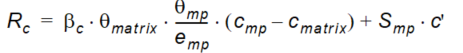
The source/sink term, Rc, describing solute exchange between matrix and macropores is given by a combination of a diffusion component and a mass flow component

Equation 36.20

where - \(b_c\) is a mass transfer coefficient - \(c_{mp}\) and \(cmatrix\) are the solute concentrations in the macropores and matrix, respectively, - \(c\) is the concentration in either matrix or macropores depending on the direction of the exchange flow, \(Smp\).

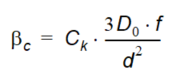
The mass transfer coefficient, \(b_c\), can be derived from

Equation 36.21

where - \(C_k\) is the dimensionless contact factor to take care of an eventual coating at the interior walls of the macropores. The contact factor ranges from 0.0 (no contact) to 1.0 (full contact). - \(D_0\) [m2/s] is the diffusion coefficient in free water of the solute species. - \(f\) is a dimensionless impedance factor that represents and decreases with the tortuosity of the macropores. f ranges from 0.0 (zero diffusivity) to 1.0 (full diffusivity). Thereby, bc depends on both solute species and soil type.

Even though the applied macropore description can be regarded as mechanistic with parameters having physical meaning, some of the parameters required to characterise the macropore system are either difficult or impossible to measure. This is particularly the case for the parameters regulating exchange between matrix and macropores. Field observations of soil structure and the occurrence of biotic macropores can give indications of the mass exchange parameters (Jarvis et al., 1997; Jarvis, 1998), though recent experiences reveal that parameters obtained from such macroscopic observations often need adjustments towards longer diffusion lengths when applied to field measurements (Saxena et al., 1994; Larsson and Jarvis, 1999). The main reason for this is expected to be organic and clay coatings on the aggregate surfaces which reduce mass exchange rates between the two domains (Thoma et al., 1992; Vinther et al., 1999).

c. Solution Scheme

Similar to the saturated zone, the unsaturated solute transport is solved explicitly, using upstream differencing for the advection term and central differencing for the dispersion term.

Neglecting the dispersion terms and the source/sink term and assuming that the flow field satisfies the equation of continuity and varies uniformly within a grid cell, the advection component is

Equation 36.22

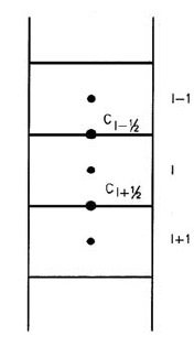
Figure 36.5 Control volume defining an internal grid.

For the control volume shown in Figure 36.5, this equation is written in finite difference form as:

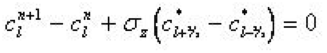
Equation 36.23

where - \(n\) denotes the time index - \(c_l\) is the concentration in the computational node - \(c\) is the interpolated concentration at the edges of the grid at time n - \(\sigma_z\) is the directional Courant number defined by

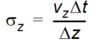
Equation 36.24

As the c*-terms are not located at the nodal points, they have to be interpolated from known concentration values. The equation for this follows the one derived for the saturated zone

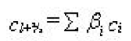
Equation 36.25

However, in the unsaturated zone only three weights need to be determined

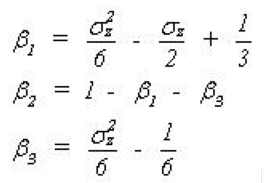
Equation 36.26

where the weights are positioned relative to the actual flow direction.

Dispersive transport can be derived in a similar way. If the finite difference formulation of the dispersive transport is based on upstream differencing in concentration and central differencing in the dispersion coefficients, the dispersive transport is

Equation 36.27

The dispersive transport is incorporated into the weights.

The above solution is strictly speaking only valid for a regular discretisation but if the resolution varies slowly the error introduced is small.

d. Initial Conditions

The initial concentration in the unsaturated zone is given as average concentrations. The unit for the concentration is [mass/volume]. This way of giving the initial conditions has the advantage that you does not have to worry about the vertical discretisation and the water content. On the other hand, you do not know the exact amount of mass introduced into the unsaturated zone, since this depends on the initial water content determined in the water movement simulation.

e. Source/Sinks, Boundary Conditions and other Exchanges

Sources for solute input into the unsaturated zone can be given in a number of ways both as point or line sources at specific depth intervals or as area sources at specific locations.

Dissolved matter can enter the unsaturated zone in three different ways. It can either be added to the precipitation as a so-called precipitation source (if the overland part is not included in the simulation) or it can be a UZ-source introduced at a certain depth or it can enter from the saturated zone. The precipitation source option is described in the section about Overland Solute Transport.

The unsaturated zone transport component exchanges mass with the overland and the groundwater transport components as indicated in Figure 2. The transport from the overland component is a one way transport from the overland to the unsaturated zone whereas both transport to and from the groundwater can occur.

Point and line sources can be included with units of [mass/time]. Spatially distributed sources can be included with units of [mass/area/time]. In each calculation time step the solute mass in all grids nodes is updated with mass from the source.

It is not possible to introduce external sinks in the unsaturated zone. However, water can be removed by the roots or via soil evaporation, which can consequently increase solute concentrations.

4. Solute Transport in Overland Flow

MIKE SHE calculates the movement of solutes in overland flow, when ever ponded water exists. In surface water the mixing and spreading of solutes is mainly due to turbulence, which appears when the flow velocity exceeds a certain level. This process is known as turbulent diffusion and is generally far more important than molecular diffusion.Although this process is physically different from the spreading of solutes in groundwater, solute transport in surface water is usually still described using the advection-dispersion equation. Similar to the saturated zone, the 2D advection-dispersion equation for overland transport is solved using the explicit, third-order accurate QUICKEST scheme.

As for solute transport in the saturated zone, the dispersion coefficients depend on the spatial and temporal scale of averaging. However, dispersion in surface water depends on the homogeneity of the velocity distribution in the flow cross-section. To some extent, the dispersion depends on the mean flow velocity. However, there is no general dependence between the dispersion coefficient and the mean flow velocity. Therefore, in surface water models, the dispersion coefficient is usually specified directly. In MIKE SHE, the dispersion coefficients are assumed constant in time but may vary in space.

a. Governing Equations

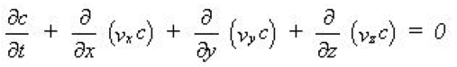
The transport of solutes on the ground surface is governed by the two-dimensional advection-dispersion equation

Equation 36.28

where - \(c\) is the concentration of the solute - \(R_c\) is sum of sources and sinks - \(D_{ij}\) is the dispersion tensor - \(v_i\) is the velocity tensor.

The velocity of water is determined from the water flux and water depth calculated during the WM simulation.

For overland transport the longitudinal and transverse dispersion coefficients (\(D_L\) and \(D\)) are specified directly and the dispersion coefficients applied in Eq. (36.28) are determined as for isotropic conditions in groundwater as

Equation 36.29

The water depth on the ground surface varies in space and time, due to variations in topography, as well as variations in precipitation, evaporation, infiltration etc. Since evaporation can concentrate a solute beyond its solubility, a mass balance of precipitated solute is maintained, where the solute will redissolve if additional water becomes available. The precipitation and dissolution of the solute is controlled by its solubility.

b. Solution scheme

The solution scheme applied for overland transport uses the same QUICKEST scheme as in the saturated zone. It is a fully explicit scheme that using upstream differencing.

Neglecting the dispersion terms and the source/sink term and assuming that the flow field satisfies the equation of continuity and varies uniformly within a grid cell, the advection-dispersion equation can be written as

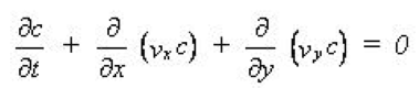
Equation 36.30

and when written in finite difference form becomes

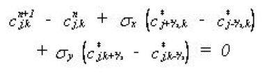
Equation 36.31

where - \(n\) denotes the time index.

In Eq. (36.31), \(\sigma_x\) and \(\sigma_y\) are the directional Courant numbers defined by

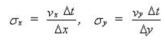
Equation 36.32

and the c-terms are the concentrations at the surface of the control volume at time n*. As these terms are not located at nodal points, they are interpolated from known concentration values by

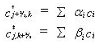
Equation 36.33

The concentration \(ci\) is the concentration around the actual point, for example (j-1,k) and the weights \(\delta_i\) and \(\delta_i\) are determined in such a way that the scheme becomes third-order accurate. The determination of the weights is demonstrated in Vested et al. (1992) and listed in Table 36.3. The other “boundary” concentrations are found in a similar way.

Table 36.3 Weight functions for advective transport

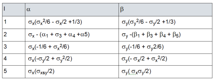
The locations of the weights are determined by the points that enter into the discretisation. Since the scheme is upstream centred, the weights are positioned relative to the actual direction of the flow. This is outlined in more detail for in the saturated zone Solution Scheme section.

The dispersive transport can be derived in a similar way. With the finite difference formulation of the dispersive transport components based on upstream differencing in concentrations and central differencing in dispersion coefficients, the transport in the x-direction can be written as

Equation 36.34

The dispersive transport in the y direction is done in a similar way. The dispersive transports are incorporated in the weight functions, so that the mass transports can be calculated in one step.

c. Initial Conditions

The initial concentration can be a fully distributed concentration field (e.g. measured or simulated concentrations at a certain time). The unit for the overland concentration is [mass/area].

If there is a flux of water into the model area from boundary points the flux concentration in these points will be constant in time and equal to the initial concentration, if the flux concentration at any of these points is not specified as a time-varying source concentration.

d. Source/Sinks, Boundary Conditions and other Exchanges

Dissolved solutes can be added to the overland flow via precipitation, or from discharging groundwater. Alternatively, the solute can be added directly as a spatially distributed source on the land surface.

As indicated in Figure 36.2 the overland transport component exchanges mass with the river, the unsaturated zone and the saturated zone. In the case of exchange to the river, the solute mass is simply added as a source term to

MIKE 1D. Similarly, infiltration is added as a source in the unsaturated zone. Exchange directly to the saturated zone can occur, if by-pass flow is allowed, in which case, the bypass flow concentration is the same as the concentration in the overland flow. Exchange to overland flow from the saturated zone occurs if the water table rises above the ground surface.

A spatially distributed source is specified using a dfs2 file, where the source strength is given in units of [mass/area/time].

It is not possible to introduce external sinks for overland transport. However, solute concentrations can increase due to evaporation.

6. Solute Transport in MIKE 1D

In MIKE SHE, the solute transport in the river channels is handled by the MIKE 1D Advection-Dispersion (AD) module.

In MIKE 1D, the 1D advection-dispersion equation is solved using an implicit finite difference scheme that is, in principle, unconditionally stable with negligible numerical dispersion. A correction term has been added to reduce the third-order truncation error, making it possible to simulate very steep concentration gradients.

Longitudinal dispersion in channels is largely controlled by the non-uniform velocity distribution both spatially and temporally. In rivers the dispersion coefficient is normally on the order of 5 to 10 m2/s increasing to between 30 and 100 m2/s when 2D processes, such as secondary currents and wind induced turbulence begin to dominate.

MIKE 1D exchanges solutes with MIKE SHE’s overland and saturated zone flow components.

Detailed information on this module is available as part of the MIKE+ River Network Modelling technical documentation.