Sorption and Decay
1. Water Quality Sorption and Decay
| WQ Sorption and Decay | |
|---|---|
| Conditions | if the option Include Advection Dispersion (AD) Water Quality is selected in the Simulation Specification dialogue and Include Water Quality Processes is turned on in the Water Quality Simulation Specification dialogue |
The Sorption and Decay dialogue appears when you have turned on the Water Quality Processes option.
Decay Processes
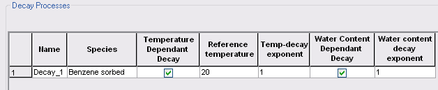
Temperature dependent decay
It means that the rate of decay increases when the temperature is above a reference temperature and decreases when below. For overland flow, the ponded water is assumed to have the same temperature as the air. For the unsaturated and saturated zones, the soil temperature is dynamically calculated based on the air temperature.
Reference Temperature
This is the reference temperature for the decay function in Equation(37.15).
Temp Decay Exponent
This is the decay exponent, \(\alpha\), in Equation (37.15).
Water content decay
It means that the actual rate of decay changes depending on the actual water content in the unsaturated zone relative to the saturated water content.
Water Content Decay Exponent
This is the decay exponent, \(\beta\), in Equation(37.14).
Sorption Processes
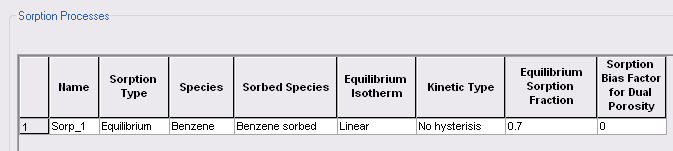
Sorption type
The sorption type can be Equilibrium or Equilibrium-Kinetic. In the first case, the sorption is assumed to be instantaneous. In the second case, the sorption is rate dependent.
However, the solute is divided into an equilibrium fraction and a kinetic fraction, which defined by the value specified in the Equilibrium Sorption Fraction column. If the kinetic option is selected, then a kinetic rate constant will be added in the relevant Sorption process data tree items in the Unsaturated and Saturated sub-trees.
Species
This is the name of the species that will be sorbed. The combo box includes only of the dissolved species listed in the main Species dialog.
Sorbed Species
This is the name of the sorbed version of the dissolved species. This combo box includes only the sorbed species from the Species dialog.
Equilibrium Isotherm
The equilibrium isotherm can be either a Linear isotherm, or one of two non-linear isotherms: Freundlich or Langmuir. The selection of the particular sorption isotherm will create different data tree sub-items for the isotherm parameters, as described below.
Linear sorption isotherm
It is mathematically the simplest isotherm and can be described as a linear relationship between the amount of solute sorbed onto the soil material and the aqueous concentration of the solute, where Kd is known as the distribution coefficient.
Freundlich sorption isotherm
It is a more general equilibrium isotherm, which can describe a non-linear relationship between the amount of solute sorbed onto the soil material and the aqueous concentration of the solute, where K and N are constants.
Both the linear and the Freundlich isotherm suffer from the same fundamental problem. That is, there is no upper limit to the amount of solute that can be sorbed. In natural systems, there is a finite number of sorption sites on the soil material and, consequently, an upper limit on the amount of solute that can be sorbed.
Langmuir sorption isotherm
It takes this into account. When all sorption sites are filled, sorption ceases. For the Langmuir sorption isotherm \(\alpha\) is a sorption constant related to the binding energy and \(\alpha\) is the maximum amount of solute that can be absorbed by the soil material.
For more details on the sorption isotherms, see Equilibrium Sorption Isotherms.
Kinetic Type
The three equilibrium sorption isotherms described above can be extended to include kinetically controlled sorption. In the MIKE SHE AD module, a two-domain approach is used, where the sorption is assumed to be instantaneous for a fraction of the sorbed solute and rate-controlled for the remainder. (see below). If Equilibrium-Kinetic is selected in this combo box, then an additional data tree sub-item will be added in the UZ and SZ WQ sections for the kinetic rate constant specified in Equation (37.9).
Equilibrium Sorption Fraction
This is the fraction of solute that is sorbed instantaneously using the equilibrium isotherm. The remainder is sorbed more slowly based on the kinetic rate constant.
Sorption Bias Factor for Dual Porosity
Sorption depends on the porosity and the bulk density of the soil. In dual porosity systems this is rather complicated. The distribution of sorption between the matrix and the fractures should be calculated based on the bulk density and different porosities. However, this is not always practically possible, so MIKE SHE includes a sorption bias factor that allows you to explicitly control the sorption distribution between the fractures and the matrix. The sorption bias factor function is shown in Figure 37.3.
- Sorption bias factor = - 1 Sorption is only in the matrix region.
- Sorption bias factor = 0 The distribution of sorption sites between macro pores and matrix is assumed to be proportional to the distribution of porosities.
- Sorption bias factor = 1 Sorption is only in the macro pores.
Related Items:
- Working with Solute Transport - User Guide
- Advection Dispersion - Reference
- Reactive Transport - Reference
2. Water Quality Decay Processes
If WQ in unsaturated flow is to be calculated, then each decay process specified in the Water Quality Sorption and Decay dialog will add one item to this data tree branch, with the name equal to that specified in the dialog.
Each branch will include the first-order decay half-life for the species specified in the decay process.
a. Half Life
| Half Life | |
|---|---|
| Condition | when Water quality processes are selected in the Water Quality Simulation Specification dialogue AND at least one decay process is active. |
| dialogue Type | Stationary Real Data |
| EUM Data Units | Half-life |
The half-life equals the length of time for half of the current solute to disappear. For rapidly decaying solutes a typical half-life could be a few days to a few months. For slowly decaying species this could be a few years to many centuries. But, for long-lived radioactive elements the half-life can be 10000 years or more.
Related Items:
- Water Quality Sorption and Decay
- Solute Transport in Overland Flow
- Solute Transport in the Unsaturated Zone
- Solute Transport in the Saturated Zone
b. Macropore/Secondary Half Life
| Macropore/Secondary Half Life | |
|---|---|
| Condition | when Water Quality processes are selected in the Water Quality Simulation Specification dialogue AND at least one decay process is active AND Full Macropore Flow selected in the main Unsaturated dialog OR Transfer to immobile water selected for SZ |
| dialogue Type | Stationary Real Data |
| EUM Data Units | Half-life |
The half-life equals the length of time for half of the current solute to disappear. For rapidly decaying solutes a typical half-life could be a few days to a few months. For slowly decaying species this could be a few years to many centuries. But, for long-lived radioactive elements the half-life can be 10000 years or more.
The decay half-life in macropores may or may not be the same as in the bulk media. For example, water in the macropores may be more oxygenated.
Related Items:
- Water Quality Sorption and Decay
- Solute Transport in Overland Flow
- Solute Transport in the Unsaturated Zone
- Solute Transport in the Saturated Zone
3. Water Quality Sorption processes
If WQ in unsaturated flow is to be calculated, then each sorption process specified in the Water Quality Sorption and Decay dialog will add one item to this data tree branch, with the name equal to that specified in the dialog. Each branch will include the appropriate sorption coefficients for the selected sorption isotherm for the species specified in the sorption process.
a. Linear Kd
| Linear Kd | |
|---|---|
| Condition | when water quality for Unsaturated or Saturated flow is selected in the Water Quality Simulation Specification dialogue and the Linear Isotherm is selected for the sorption process |
| dialogue Type | Stationary Real Data |
| EUM Data Units | Kd |
The linear sorption isotherm is mathematically the simplest isotherm and can be described as a linear relationship between the amount of solute sorbed onto the soil material and the aqueous concentration of the solute:
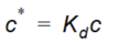
Equation 11.09
where \(K_d\) is known as the distribution coefficient.
The distribution coefficient is often related to the organic matter content of the soil by an experimentally determined parameter (Koc) which can be used to calculate the Kd values.
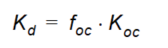
Equation 11.10
where \(f_{oc}\) is the fraction of organic carbon.
Commonly referred to is the retardation factor (R), which is the ratio between the average water flow velocity (v) and the average velocity of the solute plume (vc). The retardation factor is calculated as
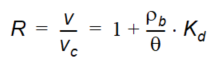
Equation 11.11
Related Items:
- Water Quality Sorption and Decay
- Solute Transport in the Unsaturated Zone
- Solute Transport in the Saturated Zone
- Equilibrium Sorption Isotherms
b. Freundlich Kf and N
| Freundlich Kf and N | |
|---|---|
| Condition | Condition when water quality for Unsaturated or Saturated flow is selected in the Water Quality Simulation Specification dialogue and the Freundlich Isotherm is selected for the sorption process |
| dialogue Type | Stationary Real Data |
| EUM Data Units | Kd and Dimensionless exponent |
The Freundlich sorption isotherm is a more general equilibrium isotherm, which can describe a non-linear relationship between the amount of solute sorbed onto the soil material and the aqueous concentration of the solute
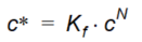
Equation 11.12
where \(K_f\) and N are constants. The relationship between K and N is shown in Figure 37.1.
Related Items:
- Water Quality Sorption and Decay
- Solute Transport in the Unsaturated Zone
- Solute Transport in the Saturated Zone
- Equilibrium Sorption Isotherms
c. Langmuir alpha and beta
| Freundlich Kf and N | |
|---|---|
| Condition | when water quality for Unsaturated or Saturated flow is selected in the Water Quality Simulation Specification dialogue and the Langmuir Isotherm is selected for the sorption process |
| dialogue Type | Stationary Real Data |
| EUM Data Units | Kd and Concentration_4 |
Both the linear and the Freundlich isotherm suffer from the same fundamental problem. That is, there is no upper limit to the amount of solute that can be sorbed. In natural systems, there is a finite number of sorption sites on the soil material and, consequently, an upper limit on the amount of solute that can be sorbed. The Langmuir sorption isotherm takes this into account. When all sorption sites are filled, sorption ceases. The Langmuir isotherm is often given as
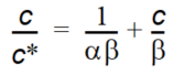
Equation 11.13
Or
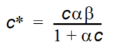
Equation 11.14
where \(\alpha\) is a sorption constant related to the binding energy and \(\beta\) is the maximum amount of solute that can be absorbed by the soil material. The relationship between \(\alpha\) and \(\beta\) is shown in Figure 37.2.)
Related Items:
- Water Quality Sorption and Decay
- Solute Transport in the Unsaturated Zone
- Solute Transport in the Saturated Zone
- Equilibrium Sorption Isotherms
d. Kinetic Sorption/Desorption Rate
| Kinetic Sorption Rate | |
|---|---|
| Condition | when water quality for Unsaturated or Saturated flow is selected in the Water Quality Simulation Specification dialogue AND at least one active Sorption process is using the Kinetic/Equilibrium isotherm option |
| dialogue Type | Stationary Real Data |
| EUM Data Units | 1st order rate WQ model |
The kinetic sorption rate is the specified rate at which the solute is absorbed onto the soil matrix. The kinetic rate is used whenever a kinetic sorption isotherm is specified.
The kinetic desorption rate is the specified rate at which the solutes go back into solution from the soil matrix. The desorption rate is used whenever hysteresis is allowed for the kinetic sorption isotherm is used.
Related Items: