Storing of Results
1. Overview
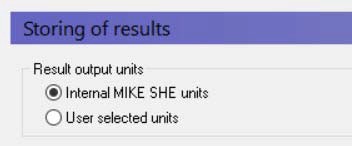
Result Output units - By default, the output files are created using the internal MIKE SHE SI units. To support Imperial (American) units, the output files can be optionally output in the units as defined under the menu: File/Options/Edit Unit Base Groups...
a. Water Movement Output
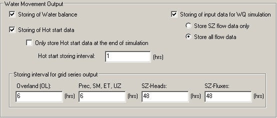
Storing of water balance data
When this option is selected, MIKE SHE will store all of the relevant output data for the analysis of the water balance. This will automatically select the required items in the Grid Series Output section.
Storing of Hot start data
The option allows you to save a simulation that can be used as the start a new simulation. See Time Step Control for more information on using Hot Start data as the initial data for a simulation.
Only store hot start data at the end of the simulation
Typically, the follow-on simulation starts at the end of the previous simulation. However, if you want to test the sensitivity of the results to the starting condition, for example, you may want to save hot start data more frequently. However, the hot start file can become very large if the hot start data is saved frequently.
Store AD input data during water movement simulation
A MIKE SHE water quality simulation is calculated based on the cell-by-cell water fluxes calculated by the water movement module. If water quality is included in the model setup, then the necessary data is automatically saved, and this item is hidden. However, if water quality is not included in the simulation, you can optionally tell MIKE SHE to save the necessary data for the water quality model by checking this box on and selecting the save option. The first option only saves the saturated zone data, which is suitable if you are only going to calculate the water quality in the saturated zone. For example, the random walk particle tracking is only available in the saturated zone and there is, therefore, no need to save overland flow data for a particle tracking simulation. The second option saves all of the data necessary for a water quality simulation in the complete integrated model.
b. Storing interval for grid series output
Gridded output can create very large output files if the data is stored at every time step. Gridded data is not usually compared to frequent measurements, such as daily groundwater levels, so the output frequency can be much less than the time step length. In fact, the output frequency of gridded output is often determined by visualization needs, such as to make smooth animations.
The gridded output for the different processes can be saved at different frequencies - the overland frequency is separate from unsaturated zone frequency is separated from the saturated zone frequency. However, you cannot save individual items at different frequencies. Thus, since precipitation, evapotranspiration and unsaturated flow output items are related, they are all saved at the same frequency. The saturated zone heads and fluxes are separated into different frequencies, however, because the gridded output files for a detailed 3D model can get very large.
Note
The Storing Time Step for SZ must be an integer multiple of the Maximum Allowed SZ Time Step that is specified in the Time Step Control dialogue. In other words, if the Maximum allowed SZ time step is 24 hours, then the Storing Time Step for SZ can only be a multiple of 24 hours (e.g. 24, 48, 72 hours, etc.).
Similarly, the storing frequency for SZ Fluxes must be an integer multiple of the SZ heads frequency, and the storing frequency for overland flow and unsaturated flow items, must be an integer multiple of their respective maximum allowed time step length.
c. Water Quality Output
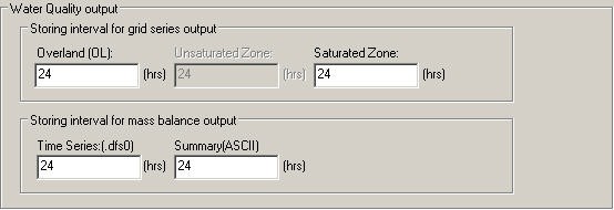
Storing interval for grid series output
similar to the storing interval for water movement data, the gridded output data files for a detailed transport simulation can get very large. These three frequencies allow you to save only the data you need.
Storing interval for mass balance output
similar to the storing interval for grid series output, these separate storing frequencies allow you to save only the data you need.
d. Particle Tracking Output
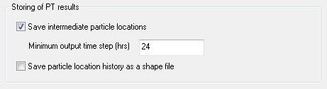
Save intermediate particle locations
If you want to plot path lines, then you need to turn this option on. You should be careful, when using this option, as the file size can easily become very large.
Minimum output time step
This value determines how often the particle locations will be saved. The more frequent the saving, the larger the output file.
Save particle location history as a shape file
The intermediate points can be saved directly into a shape file. However, since there can be hundreds or even thousands of particles in a PT simulation, this can generate very large shape files.
Related Items:
2. Detailed WM time series output
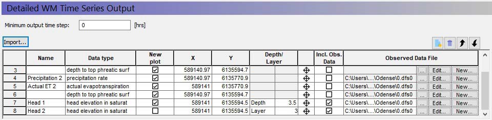
The Detailed time series output dialogue allows you to specify the location at which you want detailed time series output and the item that you want output. For each specified point, the output variable is stored in a .dfs0 file with one value for every simulation time step. Finally, for each item in the detailed time series table, an HTML plot is created in the Result Tab.
Note
All of the detailed time series items are stored in one .dfs0 file. This can lead to file size and disk space errors, if you have a long detailed simulation or more than \~200 detailed time series items. Also, the display in the Results Tab will become very slow if you have a lot of items, since it has to read the entire .dfs0 file and generate all of the graphs every time you access the Detailed Time Series page in the Results Tab.
Minimum Output time step*
In some simulations, the output time step can become very small due to the automatic time step adjustment. If the output is being saved every simulation time step, then the output files can become very large. This value allows you to set a lower limit on the output time step. Note, however, that the sub-time step values are averaged over the Minimum output time step.
Name
This is a text field that can be used to specify a reference name for the location, for example, a borehole name. This is also the name that will be used for the time series item in the Dfs0 file created during the simulation.
Data Type
This is the list of available output items is dynamic in the sense that the list changes in response to the processes included in the Simulation Specification dialogue. Further, additional items are available that are related to simulation variables, such as the number of iterations during each Saturated Zone time step. A list of available Data Types can be found in Output Items.
New plot
If this is checked, then a new detailed time series HTML-plot will be created on the Results Tab. If this is unchecked, then the output will be added to the previous plot. You can use the Up and Down arrows to arrange the output points so that relevant points are plotted together.
X, Y
Often, detailed time series are associated with measurement stations. That is, locations at which a time series of measurements are available, for example, water levels in a well or water depths on a flood plain. This is the (X, Y) map coordinates of the point in the same EUM units (ft, m, etc.) as specified in the EUM Database for Item geometry 2-dimensional. (see EUM Data Units)
Depth/Layer
This is the depth of the observation point below land surface for subsurface observation points. It can be specified either as a 1-based layer index (top down), or as a depth in the same EUM units (ft, m, etc.) as specified in the EUM Database for Depth Below Ground (see EUM Data Units).
Target Icon
You can use the target icon to locate the output point exactly. Alternatively, you can type the exact coordinates or import the items from an ASCII file.
Include observation data
If this is checked, then a .dfs0 file can be specified that includes observation points. The observation points are automatically plotted along with the results in the plot on the Results tab. The .dfs0 item is selected in the file browser dialogue. The Edit button opens the specified .dfs0 file and the New button can be used to create a new .dfs0 file with the correct item type etc. and at the same time import data from an Excel spreadsheet.
a. Importing data
Detailed MIKE SHE Time Series data can be imported directly into the Detailed MIKE SHE Time Series dialogue using the Import button. The data file must be a tab-delimited ASCII file without a header line. The file must contain the following fields and be in the format specified below.
Name>DataTypeCode>NewPlot>X>Y>UseLayer>Depth/Layer>UseObsdata>dfs0file name>dfs0ItemNumber
where the > symbol denotes the Tab character and
Name
This is the user specified name of the observation point. This is the name that will be used for the time series item in the Dfs0 file created during the simulation.
DataTypeCode
This is a numeric code used to identify the output data type. A list of available Data Type Codes can be found in Output Items.
NewPlot
This is a flag to specify whether a new detailed time series HTML-plot will be created on the Results Tab:
0 = the output will be added to the previous plot.
1 = Create a new plot
X, Y
This is the (X, Y) map coordinates of the point in the same EUM units (ft, m, etc.) as specified in the EUM Database for Item geometry 2-dimensional. (see EUM Data Units)
UseLayer
select whether the next field contains a depth (value 0) or a layer index (value 1)
Depth/Layer
This is the depth of the observation point below land surface for sub-surface observation points. It can be specified either as a 1-based layer index (top down), or as a depth in the same EUM units (ft, m, etc.) as specified in the EUM Database for Depth Below Ground (see EUM Data Units). The previous field defines whether this is a depth or a layer index.
UseObsData
This is a flag to specify whether or not an observation file needs to be input: 0 = No; 1 = Yes
dfs0file name
This is the file name of the dfs0 time series file with observation data. The path to the dfs0 file must be relative to the directory containing the MIKE SHE *.she document. The dfs0 extension is optional. If it is not included, it will be added to the file name automatically. For example,
.\Time\Calibration\GroundwaterObs
refers to the file GroundwaterObs.dfs0 located in the subdirectory Time\Calibration, which is found in the same directory as the .she model document.
dfs0ItemNumber
This is the Item number of the observation data in the specified DFS0 file.
The following is a simple example with three MIKE SHE observation points, where the file name is obsdata.dfs0.
OL depth 61 GrandRiver 34500 18300 0
CZ head 1 101 GrandRiver 34500 18300 0 5.5 1 .\time\obsdata.dfs0 1
CZ Head 2 101 GrandRiver 34500 18300 1 4 1 .\time\obsdata.dfs0 2
Related Items:
- Time Step Control
- Detailed River Time Series Output
- Grid series output
- MIKE SHE Detailed Time Series
3. Detailed WQ time series output
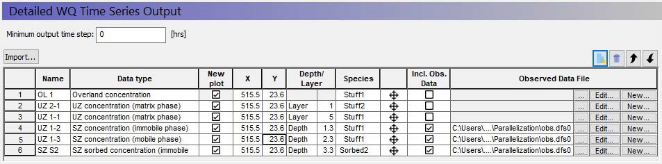
The Detailed WQ Time Series output dialogue allows you to specify the location at which you want detailed time series output of concentrations. For each specified point, the output variable is stored in a .dfs0 file with one value for every simulation time step. Finally, for each item in the detailed time series table, an HTML plot is created in the Result Tab.
Note
All of the detailed time series items are stored in one .dfs0 file. This can lead to file size and disk space errors, if you have a long detailed simulation or more than \~200 detailed time series items. Also, the display output in the Results Tab will become very slow if you have a lot of items, since it has to read the entire .dfs0 file and generate all of the graphs every time you access the Detailed Time Series page in the Results Tab.
Minimum Output time step
In some simulations, the output time step can become very small due to the automatic time step adjustment. If the output is being saved every simulation time step, then the output files can become very large. This value allows you to set a lower limit on the output time step. Note, however, that the sub-time step values are averaged over the Minimum output time step.
Name
This is a text field that can be used to specify a reference name for the location, for example, a borehole name. This is also the name that will be used for the time series item in the Dfs0 file created during the simulation.
Data Type
This is the list of available output items. It is dynamic in the sense that the list changes in response to the processes included in the Water Quality Simulation Specification dialogue. A list of available Data Types can be found in MIKE SHE Output Items.
New plot
If this is checked, then a new detailed time series HTML-plot will be created on the Results Tab. If this is unchecked, then the output will be added to the previous plot. You can use the Up and Down arrows to arrange the output points so that relevant points are plotted together.
X, Y
Often, detailed time series are associated with measurement stations. That is, locations at which a time series of measurements are available, for example, water levels in a well or water depths on a flood plain. This is the (X, Y) map coordinates of the point in the same EUM units (ft, m, etc.) as specified in the EUM Database for Item geometry 2-dimensional. (see EUM Data Units)
Depth/Layer
This is the depth of the observation point below land surface for subsurface observation points. It can be specified either as a 1-based layer index (top down), or as a depth in the same EUM units (ft, m, etc.) as specified in the EUM Database for Depth Below Ground (see EUM Data Units).
Species
This is the list of Species in the WQ simulation.
Target Icon
You can use the target icon to locate the output point exactly. Alternatively, you can type the exact coordinates or import the items from an ASCII file.
Include observation data
If this is checked, then a .dfs0 file can be specified that includes observation points. The observation points are automatically plotted along with the results in the plot on the Results tab. The .dfs0 item is selected in the file browser dialogue. The Edit button opens the specified .dfs0 file and the New button can be used to create a new .dfs0 file with the correct item type etc. and at the same time import data from an Excel spreadsheet.
a. Importing data
Detailed MIKE SHE Time Series data can be imported directly into the Detailed MIKE SHE Time Series dialogue using the Import button. The data file must be a tab-delimited ASCII file without a header line. The file must contain the following fields and be in the format specified below.
Name>DataTypeCode>NewPlot>X>Y>UseLayer>Depth/Layer>UseObsdata>dfs0file name>dfs0ItemNumber
where the > symbol denotes the Tab character and
Name
This is the user specified name of the observation point. This is the name that will be used for the time series item in the Dfs0 file created during the simulation.
DataTypeCode
This is a numeric code used to identify the output data type. A list of available Data Type Codes can be found in MIKE SHE Output Items.
NewPlot
This is a flag to specify whether a new detailed time series HTML-plot will be created on the Results Tab:
0 = the output will be added to the previous plot.
1 = Create a new plot
X, Y
This is the (X, Y) map coordinates of the point in the same EUM units (ft, m, etc.) as specified in the EUM Database for Item geometry 2-dimensional. (see EUM Data Units)
UseLayer
select whether the next field contains a depth (value 0) or a layer index (value 1)
Depth/Layer
This is the depth of the observation point below land surface for subsurface observation points. It can be specified either as a 1-based layer index (top down), or as a depth in the same EUM units (ft, m, etc.) as specified in the EUM Database for Depth Below Ground (see EUM Data Units). A depth value must always be included.
Species
This is the name of the species to be used.
UseObsData
This is a flag to specify whether or not an observation file needs to be input: 0 = No; 1 = Yes
dfs0file name
This is the file name of the dfs0 time series file with observation data. The path to the dfs0 file must be relative to the directory containing the MIKE SHE *.she document. The .dfs0 extension is optional. If it is not included, it will be added to the file name automatically. For example,
.\Time\Calibration\GroundwaterObs
refers to the file GroundwaterObs.dfs0 located in the subdirectory Time\Calibration, which is found in the same directory as the .she model document.
dfs0ItemNumber
This is the Item number of the observation data in the specified DFS0 file.
The following is a simple example with three MIKE SHE observation points, where the file name is obsdata.dfs0.
OL conc 216 GrandRiver 34500 18300 Species 1 0
CZ conc 1 101 GrandRiver 34500 18300 0 Species 2 1 .\time\obsdata.dfs0 1
CZ conc 2 101 GrandRiver 34500 18300 1 Species 3 1 .\time\obsdata.dfs0 2
Related Items:
- Time Step Control
- Detailed River Time Series Output
- Grid series output
- MIKE SHE Detailed Time Series
4. Detailed River Time Series Output
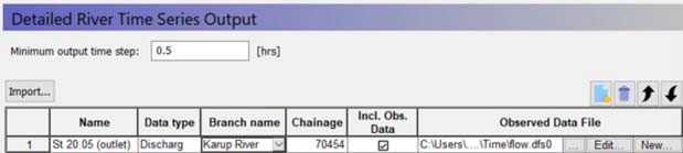
The Detailed time series output for the river allows you to specify the river chainage location at which you want detailed time series output and the item that you want output. For each specified point, the output variable is stored in a .dfs0 file with one value for every simulation time step. Finally, for each item in the detailed time series table, an HTML plot is created in the Result Tab - with or without observation data.
The principal advantage of this option is that you can now easily create calibration plots of calculated versus observed water levels without opening and having to create specific plots in MIKE View.
Minimum Output time step
In some simulations, the output time step can become very small due to the automatic time step adjustment. If the output is being saved every time step, then the output files can become very large.
This value allows you to set a lower limit on the output time step. Note, however, that the sub-time step values are averaged over the Minimum output time step.
Name
This is a text field that can be used to specify a reference name for the location, for example, a gage name.
Data Type*
This is the list of available output items, which for MIKE 1D only contains two items - water level and flow rate.
Branch name
the Branch name must be a valid branch name in the river model. However, this is not checked until run time, at which point an error message will be generated if it is not valid and the simulation will be stopped.
Chainage
like the branch name, the chainage must be a valid river chainage.
Include observation data
If this is checked, then a .dfs0 file can be specified that includes observation points. The observation points are automatically plotted along with the results in the HTML plot on the Results tab. The .dfs0 item is selected in the file browser dialogue. The Edit button opens the specified .dfs0 file and the New button can be used to create a new .dfs0 file with the correct item type etc. and at the same time import data from an Excel spreadsheet.
a. Importing data
Detailed River Time Series data can be imported directly into the dialogue using the Import button. The data file must be a tab-delimited ASCII file without a header line. The file must contain the following fields and be in the format specified below.
Name>DataTypeCode>BranchName>Chainage>UseObsdata>dfs0file name>dfs0ItemNumber
where the > symbol denotes the Tab character and
Name
The user specified name of the observation point. This is the name that will be used for the time series item in the Dfs0 file created during the simulation.
DataTypeCode
This is a numeric code used to identify the output data type: 0 for Water Level and 1 for Discharge.
Branch name
the Branch name must be a valid branch name in the river model. However, this is not checked until run time, at which point an error message will be generated if it is not valid and the simulation will be stopped.
Chainage
like the branch name, the chainage must be a valid river chainage.
UseObsData
This is a flag to specify whether or not an observation file needs to be input: 0 = No; 1 = Yes
dfs0file name
This is the file name of the dfs0 time series file with observation data. The path to the dfs0 file must be relative to the directory containing the MIKE SHE *.she document. The .dfs0 extension is added to the file name automatically and must not be included in the file name. For example,
.\Time\Calibration\RiverstageObs
refers to the file RiverStageObs.dfs0 located in the subdirectory Time\Calibration, which is found in the same directory as the .she model document. The file name must not be empty even if UseObsData is set to 0.
dfs0ItemNumber
This is the Item number of the observation data in the specified DFS0 file.
The following is a simple example with three river observation points, where the file name is obsdata.dfs0:
Obs_1 \> ? \> GrandRiver \> 34500. \>0 \>.\\time\\obsdata \>1
Obs_2 \> ? \> GrandRiver \> 22500. \>1 \>.\\time\\obsdata \>2
Obs_3 \> ? \> GrandRiver \> 1500. \>1 \>.\\time\\obsdata \>3
Related Items:
5. Grid series output
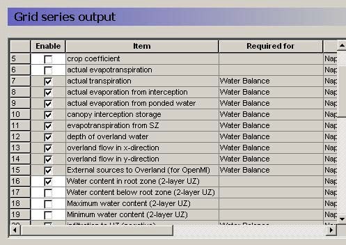
The Grid series output dialogue allows you to specify the frequency at which you want detailed output of gridded data and the items that you want output. A list of available Data Types can be found in Output Items. The list is dynamic in the sense that the list changes in response to the processes included in the Simulation Specification dialogue.
In some cases, such as when the Water Balance output has been specified (see Storing of Results), some of the items will be automatically selected and cannot be unselected. This will be noted in the Required for column of the dialogue.