Land Use
1. Introduction
The Land Use item in the data tree is used to define the items that are on the land surface that affect the hydrology in your model area, including
- Vegetation distribution, and
- Irrigation.
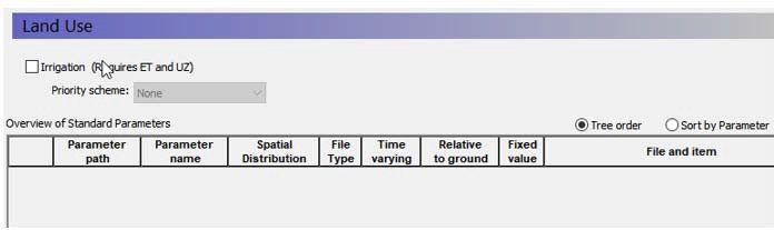
In the main menu you will also find an overview table of the main vegetation parameters used in the model. The table is blank to start with and is populated as the vegetation options and parameters are added in the sub-menus. The table of standard parameters is only active when the vegetation option from the Vegetation menu: Define Parameters Individually is selected (see section 11.14.1).
Irrigation - The Irrigation option allows you to specify a demand driven irrigation scheme with priorities. Activating the Irrigation option creates several sub-items in the data tree for the irrigation parameters. The Irrigation option requires that both Evapotranspiration and Unsaturated Flow be simulated. For more information see Irrigation Command Areas
Priority Scheme - The priority scheme is used by the Irrigation module to rank the model areas in terms of priority for irrigation. Two options are allowed: Equal Volume or Equal Shortage. If the water is to be distributed based on equal volume, then all cells with the same priority number will receive an equal amount of water, regardless of their actual demand. If the water is to be distributed based on equal shortage, then all cells with the same priority number will receive an amount of water that satisfies an equal percentage of their actual demand. For more information see Irrigation Priorities
2. Vegetation
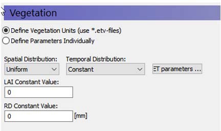
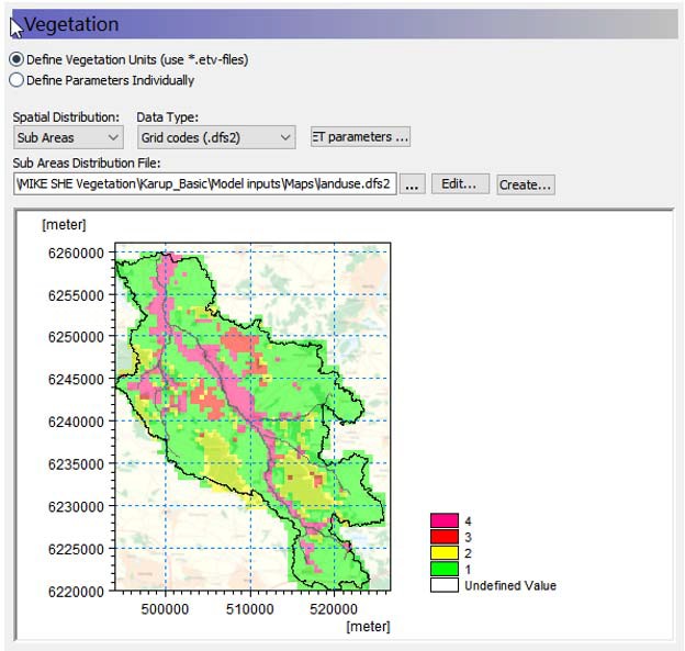
The main Vegetation dialogue is used to define the distribution of vegetation across your model area. It works the same way as the other dialogues with options for specifying constant or time varying uniform values, grid codes with associated time series or fully distributed time varying values. There are two options for specifying vegetation parameters:
- Define Vegetation Units using grids and associated time series or from a Vegetation Properties file (*.etv)
- Define Parameters Individually
2.1 Vegetation Units option
In the Define Units option there are two relevant time series parameters: the Leaf Area Index and the Root Depth. Both of these parameters can be defined as constants, via .dfs0 files, or they can be defined from a Vegetation Properties file.
If the Vegetation Properties file option is used for the Leaf Area Index and Root Depth parameters, it is possible to specify crop rotations.
Note
The crop coefficient, Kc, is only available in the Vegetation Properties file.
| Parameter | Description |
|---|---|
| Conditions | If Evapotranspiration selected in the Simulation Specification |
| EUM Data Units | Grid Code |
| Time Series EUM Data Units | Leaf Area Index and Root Depth, or Vegetation Property File (see Vegetation Properties Editor) |
| dialogue Type | Special version of Time-varying Real Data |
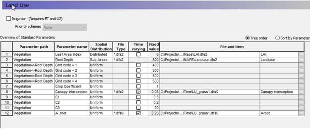
2.2 Individual Parameters option
As an alternative to the Vegetation Units option, it is possible to specify the vegetation parameters individually. This option allows you to specify the main vegetation parameters: Leaf Area Index, Root Depth and Crop coefficient individually with all available options for distributions in space and time.
Evapotranspiration parameters are also specified individually, similarly to how the vegetation parameters are specified.
An overview table of the main parameters is included in the main Land Use dialogue. From here you can also modify the input values and time series links.
2.3 Evapotranspiration Parameters
Evapotranspiration parameters are either specified through clicking on a button labelled ET Parameters... in case the Vegetation Units option is chosen, or the values are specified individually exactly like the vegetation parameters.
Clicking on the ET Parameters menu pops up the dialogue for specifying the default ET parameters.
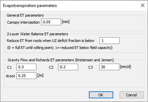
The Evapotranspiration parameters in this dialogue do not vary in time and are global for the model. However, if the Vegetation Properties file option is used for the Leaf Area Index and Root Depth parameters, these values can be overridden by crop specific evapotranspiration values specified in the vegetation properties file.
If the Individual Parameter option is chosen it is possible to specify fully distributed values in time and space for each of the evapotranspiration parameters.
The following sections are condensed from the Evapotranspiration - Technical Reference chapter, which should be consulted for more detailed information.
2.4 Canopy Interception
The interception process is modelled as an interception storage, which must be filled before stem flow to the ground surface takes place. The coefficient Cint defines the interception storage capacity of the vegetation per unit of LAI. A typical value is about 0.05 mm but a more exact value may be determined through calibration.
Note
The interception storage is calculated each time step and the rate of evaporation is usually high enough to remove all the interception storage in each time step. Thus, the total amount of water removed from interception storage depends on the length of the time step. This can lead to confusion when comparing water balances, if the time steps are different. For example, assuming it rains a little in each time step and all the interception storage is removed by ET in every time step, if the time step is halved, then the total volume of interception storage removed will double.
2.5 Deficit Fraction for reduced ET (2-Layer ET only)
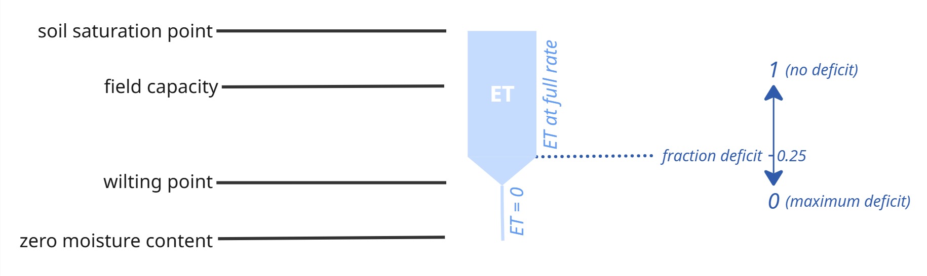
In nature, plant roots will remove water from the soil until the water content of the soil reaches a critical level. Once this level is reached, transpiration will decrease with decreasing water content until the wilting point is reached, where the amount of transpiration drops to zero.
In the 2-layer model, the maximum deficit is (\(\theta_{max}\) - \(\theta_{min}\)). If the water table is below the extinction depth, the maximum deficit is the field capacity minus the wilting point.
The deficit fraction is the fraction of this maximum deficit. When this deficit fraction is reached, MIKE SHE will start to reduce the rate of ET. In other words, transpiration will be removed at the full rate until this deficit fraction is reached. Then the transpiration rate will decrease linearly until \(\theta_{min}\) is reached, at which point transpiration will stop.
- A typical value for this deficit fraction is 0.5. This means that the ET will be removed from the UZ at the full rate until the deficit reaches half the maximum deficit.
- A deficit fraction of 1 (i.e. no deficit) means that ET will be start being reduced as soon as the water content falls below \(\theta_{max}\).
- A deficit fraction of 0 means that ET will not be reduced, and ET will be removed at the maximum rate until the wilting point is reached.
For more information on this variable, see the Section The 2-Layer Water Balance Method in the Technical documentation.
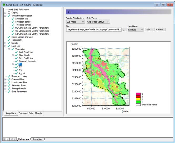
2.6 C1, C2 and C3
The Kristensen and Jensen equations for actual transpiration and soil evaporation contain three empirical coefficients, C1, C2, and C3. The coefficients C1 and C2 are used in the transpiration function, f1(LAI). C3 is the only variable found in the soil moisture function.
C1
C1 is plant dependent. For agricultural crops and grass, C1 has been estimated to be about 0.3. C1 influences the ratio soil evaporation to transpiration. This is illustrated in Figure 21.7. For smaller C1 values the soil evaporation becomes larger relative to transpiration. For higher C1 values, the ratio approaches the basic ratio determined by C2 and the input value of LAI.
C2
For agricultural crops and grass, grown on clayey-loamy soils, C2 has been estimated to be about 0.2. Similar to C1, C2 influences the distribution between soil evaporation and transpiration, as shown in Figure 21.8. For higher values of C2, a larger percentage of the actual ET will be soil evaporation. Since soil evaporation only occurs from the upper most node (closest to the ground surface) in the UZ soil profile, water extraction from the top node is weighted higher. This is illustrated in Figure 21.8, where 23 per cent and 61 per cent of the total extraction takes place in the top node for C2 values of 0 and 0.5 respectively.
Thus, changing C2 will influence the ratio of soil evaporation to transpiration, which in turn will influence the total actual evapotranspiration possible under dry conditions. Higher values of C2 will lead to smaller values of total actual evapotranspiration because more water will be extracted from the top node, which subsequently dries out faster.
Therefore, the total actual evapotranspiration will become sensitive to the ability of the soil to draw water upwards via capillary action.
C3
C3 has not been evaluated experimentally. Typically, a value for C3 of 20 mm/day is used, which is somewhat higher than the value of 10 mm/day proposed by Kristensen and Jensen (1975). C3 may depend on soil type and root density. The more water released at low matrix potential and the greater the root density, the higher should the value of C3 be. Further discussion is given in Kristensen and Jensen (1975).
2.7 Root Mass Distribution Parameter, AROOT
In the Kristensen and Jensen model, water extraction by the roots for transpiration varies over the growing season. In nature, the exact root development is a complex process, which depends on the climatic conditions and the moisture conditions in the soil. Thus, MIKE SHE allows for a root distribution determined by the root depth (time varying) and a general, vertical root-density distribution, defined by AROOT, see Figure 21.3. In the above dialogue, AROOT is not time varying, but can be specified as a time series using the Vegetation Properties Editor.
How the water extraction is distributed with depth depends on the AROOT parameter. Figure 21.4) shows the distribution of transpiration for different values of AROOT, assuming that the transpiration is at the reference rate with no interception loss (Cint=0) and no soil evaporation loss (C2=0). The figure shows that the root distribution, and the subsequent transpiration, becomes more uniformly distributed as AROOT approaches 0. During simulations, the total actual transpiration tends to become smaller for higher values of AROOT because most of the water is drawn from the upper layer, which subsequently dries out faster. The actual transpiration, therefore, becomes more dependent on the ability of the soil to conduct water upwards (capillary rise) to the layers with high root density. Figure 21.5 shows the effect of the root depth, given the same value of AROOT. A shallower root depth will lead to more transpiration from the upper unsaturated zone layers because a larger proportion of the roots will be located in the upper part of the profile. However, again, this may lead to smaller actual transpiration, if the ability of the soil to conduct water upwards is limited.
The root distribution is also important for distributing the ET extraction between the SZ and UZ models. If the water table is above the bottom of the roots then ET will be extracted from SZ. The relative amount of ET removed from SZ will depend on the fraction of roots below the water table.
Thus, AROOT is an important parameter for estimating how much water can be drawn from the soil profile under dry conditions.
2.8 Related Items
- Kristensen and Jensen method
- The 2-Layer Water Balance Method
- Vegetation Properties
- Vegetation Properties Editor
3. Vegetation Properties
| Parameter | Description |
|---|---|
| Conditions | If Evapotranspiration selected in the Simulation Specification dialogue |
| EUM Data Units | Grid Code |
| Time Series EUM Data Units | Leaf Area Index and Root Depth, or Vegetation Property File (see Vegetation Properties Editor) |
| dialogue Type | Special version of Time-varying Real Data |
There are three relevant time series parameters: the Leaf Area Index, the Root Depth and the Crop Coefficient, Kc. These parameters can be defined as constants, via .dfs0 files, or they can be defined from a Vegetation Properties file.
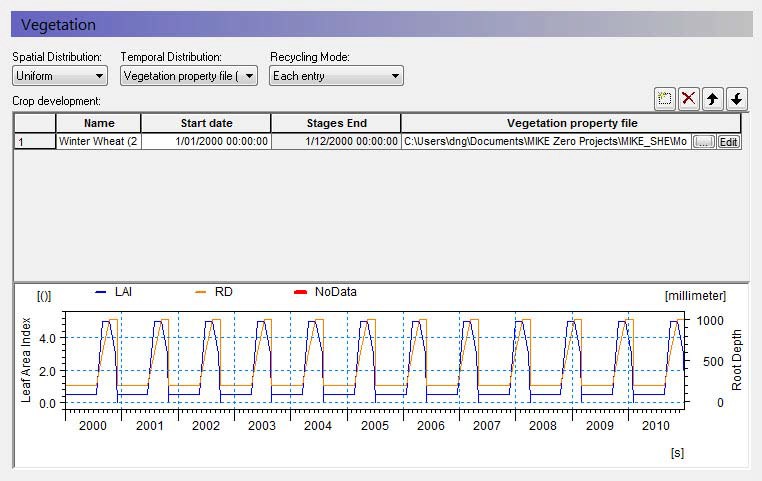
3.1 Using a Vegetation Properties file
The Vegetation Properties file typically contains a time series of the root depth and leaf area index for either one year or for the growing season. If you are using a properties file, then you have to specify the crop development schedule.
Name
This is the name of the crop or vegetation type in the properties file. This name must match exactly the name in the properties file. When you select the file name using the browse button, [...], you can select the vegetation item from a list of available vegetation types found in the file.
Start Date
The vegetation properties file typically contains information on a year or growing season basis - starting from Day 0. Thus, the Start Date is the calendar date for the beginning of the growing year or growing season. If data is missing in the time series, then the Leaf Area Index and the Root Depth are both assumed to equal zero. If the start dates overlap with the growing season information in the vegetation database, a warning will be issued in the log file that says the crop development was not over yet before the new crop was started. MIKE SHE will then start a new crop cycle at the new start date.
Tip
The times in the .etv file are instantaneous, which implies that the values between the entries are linearly interpolated. So, it is critical that you start your rotation scheme at Day 0. Otherwise, the subsequent values will all be interpolated from zero to the first rotation entry.
3.2 Recycling Mode
If you are using a Vegetation Property file, the Recycling Mode allows you to define a seasonal rotation to cover your simulation period - without having to specify a new line for each season. There are four recycling modes:
- None - if no recycling mode is defined, then you have to either specify enough lines to cover your simulation period, or that your development period in the .etv file is long enough to cover your simulation period.
- Each entry - each line will be repeated until the next start date. The last entry will be repeated until the end of the simulation
- Entire scheme - when the end of the scheme is reached, the entire scheme will start over. The scheme will repeat until the end of the simulation period. This mode requires that there are no gaps in the scheme.
- Entries, then scheme - each entry will be repeated until the start of the next entry. At the end of the scheme, the entire scheme will start over.
The Vegetation dialogue also includes a button for the Evapotranspiration Parameters, which are global stationary parameters.
3.3 Related Items
- Kristensen and Jensen method
- The 2-Layer Water Balance Method
- Vegetation Properties
- Vegetation Properties Editor
4. Irrigation Command Areas
| Parameter | Description |
|---|---|
| Conditions | Irrigation selected in Land Use and UZ and ET simulated |
| dialogue Type | Integer Grid Codes with sub-dialogue data EUM Data Units Grid Code |
| EUM Data Units | Grid Code |
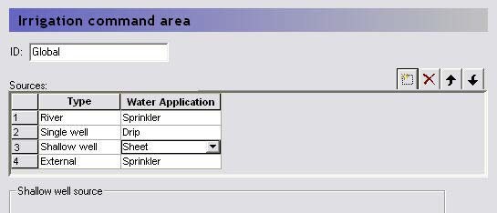
The Irrigation Command Areas are used to describe where the water comes from and how the irrigation water is applied to the model.
The Irrigation Command Area data item is divided into two dialogues. The first is the distribution dialogue for the Command Areas and the second is the Water source and Application method for each of the command areas.
Each source can also be limited by a licensed maximum amount of water in any period - License Limited Irrigation.
Calculation sequence and shortage handling for SZ Linear Reservoirs For each rank (no. of ranks = max no. of sources specified for any command area) and each Priority (usually only 1) do the following:
- Calculate the total demand of remote- and shallow well sources of the actual Rank and Priority from all baseflow reservoirs (1 & 2).
- Calculate a “supply factor” for each baseflow reservoir 1 & 2: If the demand is less than the storage of the actual reservoir, the supply factor is 1.0. Otherwise calculate a value between 0 and 1 = available storage / demand.
- Calculate the final irrigation from each source of the actual Rank and Priority = calculated demand from actual baseflow reservoir 1 and/or 2 X corresponding supply factor.
- Subtract the final irrigation volumes from the available volume of each baseflow reservoir 1 & 2 and go to next rank and priority.
In the next SZ Linear Reservoir time step, the calculated irrigation volumes are subtracted from the baseflow reservoir storages (and depths), and the irrigation pumping is stored together with the other SZLR results for water balance calculation, etc.
The available volume of water in each baseflow reservoir is calculated as
Equation 11.7:
\(V_1 = (D_r - D_w) \cdot S_y \cdot A_t \cdot F_1\)
Equation 11.8:
\(V_2 = (D_r - D_w) \cdot S_y \cdot A_t \cdot (1 - F_1)\)
where V is the available volume of water, Dr is the depth of the reservoir, Dw is the depth to the water surface in the reservoir, Sy is the specific yield of the reservoir, AT is the total surface area of the reservoir and F1 is the fraction of infiltration that is added to the first Baseflow reservoir.
4.1 Water Source Types
The Sources table specifies the different sources available for irrigation for a single command area. The order of the sources in the table is also their priority. For example, in the figure above, as long as there is sufficient water in the river, the irrigation water will be removed from the river. If the River falls below a specified level and/or discharge, then the irrigation water will be taken from the single well, and so on.
4.2 River Sources
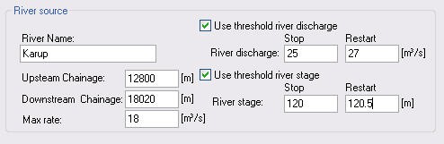
To use a river as a source of water, you must specify the river location to be used followed by the permitted river conditions that allow water to be removed. The River source actually has two conditions that can be used alone or combined.
River Name - The Branch name of the river source. This name must exist in the river model and it must be spelled correctly.
Upstream/Downstream Chainage - The upstream and downstream chainage locations to use for the river source. MIKE SHE will use the combined volume of all the included river links as the storage volume. The abstraction from each river link is volume weighted based on the total volume of the contained and partial river links.
Max rate - This is the maximum extraction rate for the river. If more water is required for irrigation, then the next source will be activated.
Use threshold river discharge - If the flow rate in the river falls below the Stop value, then water will no longer be taken from the River. However, if the flow rate in the river increases again and reaches the Restart value, the river source will be reactivated. The discharge threshold is applied at the upstream chainage location to ensure that the inflow to the river source area meets the minimum flow rate.
Use threshold river stage - If the water level in the river falls below the Stop value, then water will no longer be extracted from the River. However, if the water level in the river increases again and reaches the Restart value, the river source will be reactivated. The river stage threshold is applied at the downstream chainage to ensure that the minimum water level in the river source area is maintained.
If both threshold values are specified, then the most critical one is used, and the source will not restart until both are satisfied.
Note
There is no restriction on the number of river sources at a location. However, if the sources are located in the same model grid then a warning message will be printed to the projectname_preprocesssor_messages.log file. The sources will be merged, retaining the maximum threshold stages and the sum of the capacities. The preprocessor also checks the license application volume to make sure these are the same. If not, the preprocessor will stop with an error.
4.3 Single Well Sources
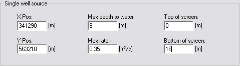
To use a well source in the model, you must specify the location and filter depth of the well. In a future release, this dialogue will be connected to the well database, but at the moment it is not.
X, Y -Pos - This is the X and Y map coordinates of the source well.
Max depth to water - this is the threshold value for the water depth in the well. If the water level in the well falls below this depth (as measured from the topography), the extraction will stop until the water level rises above the threshold.
Max rate - This is the maximum extraction rate for the well. If more water is required for irrigation, then the next source will be activated.
Top/Bottom of Screen - The depth of the top and bottom of the screen is used to define from which numerical layers water can be extracted. Pumping will stop if the water table falls below the bottom of the layer that contains the filter bottom.
There is no restriction on the number of wells at a location. However, if the wells are located in the same model grid, and have overlapping screen intervals, then a warning message will be printed to the projectname_preprocessor_messages.log file. The sources will be merged, retaining the maximum threshold depth, the sum of the capacities and the joint screening interval.
The preprocessor also checks the license application volume to make sure these are the same. If not, the preprocessor will stop with an error.
In the linear reservoir groundwater method, multiple single wells are allowed in each baseflow reservoir. No warnings are given.
When the linear reservoir method is used, the screen interval is ignored and the water is pumped from the two baseflow reservoirs. The distribution between the two reservoirs is determined by the faction give in the Baseflow Reservoirs dialogue. If the demand from one of the reservoirs exceeds the available water, the pumping will be reduced. The pumping rate at the other reservoir will not be increased to compensate.
Also in the Linear Reservoir method, the specified “max depth to water” for the actual command area and source is used. In other words, it is not using the “threshold depth for pumping” in the baseflow reservoir menu. Pumping is
allowed when the depth to the water table is less than the specified threshold value at the start of the time step.
4.4 Shallow Well Sources
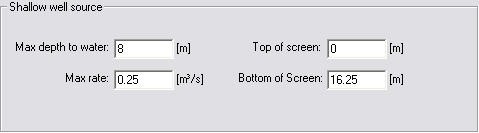
In many cases, farmers have several shallow wells for irrigation, most of which may not be mapped exactly. Especially in regional scale models, each grid cell could thus contain many shallow groundwater wells. In such cases, the Shallow Well source can be used to simply extract water for irrigation from the same cell where it is used, without having to know the exact coordinates of the wells. By specifying this option, one well is placed in each cell of the command area.
Note
A cell (i, j, layer) containing a shallow well cannot also have a single well specified in the same cell (i.e. the same cell and layer).
Max depth to water - this is the threshold value for the water depth in the well. If the water level in the well falls below this depth (as measured from the topography), the pumping will stop until the water rises above the threshold depth again.
Max rate - This is the maximum extraction rate for the shallow well in each cell. If more water is required for irrigation, then the next source will be activated.
Top/Bottom of Screen - The depth of the top and bottom of the screen is used to define from which numerical layers water can be extracted. Pumping will stop if the water table falls below the bottom of the layer that contains the filter bottom.
Shallow well sources are removed from baseflow Reservoir 1 if the Linear Reservoir groundwater method is used. The screen interval is ignored.
Note
Shallow wells can be located in cells containing single sources. The preprocessor will give a warning for such violations. Multiple shallow wells are not allowed in the same command area.
4.5 External Sources
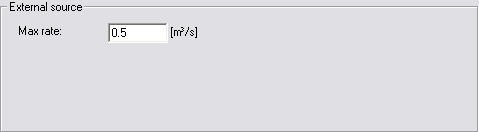
In some case, the irrigation water can be from outside of the watershed being modelled. In this case, the only constraint is the maximum amount of water than can be extracted from the source.
Max rate - This is the maximum extraction rate for the source. If more water is required for irrigation, then the next source will be activated.
4.6 Water Application methods
There are three ways to apply the irrigation water in the model.
Sprinkler - If the water is applied as sprinkler irrigation, it is added to the precipitation component.
Drip - If the water is applied as Drip irrigation, it is added directly to the ground surface as ponded water.
Sheet - If the water is applied as Sheet irrigation, then an additional data tree item is required to define where the water is to be added within the command area. The idea behind this option is that water is flooded onto one or more cells of the command area and then distributed to the adjoining cells as overland flow. The sheet irrigation is applied directly to the cells as ponded water.
All three methods are allowed in the Simple, sub-catchment based overland flow method. However, the sheet method does not really make sense if the subcatchment overland flow method is used.
4.7 License Limited Irrigation

Sometimes, the total amount of irrigation water that a user can apply is limited by a license over a certain period (e.g. 10000 m3 / year). The license limited option, allows you to specify a dfs0 time series file with a time series of maximum amounts. If the maximum amount is reached within the license period, then the irrigation will be stopped until the next license period, when it will be started again. The license period length is defined by the time steps in the specified dfs0 file.
During the simulation the license data is included in the calculation of the available water volume of each source. The module keeps track of the “actual available license volume”. Whenever this is reached or exceeded, the source will be closed until a new license period starts (or the end of the simulation). When a source is closed for this reason, a message is printed in the wm_print.log file.
Notes
- The dfs0 file EUM Data Units must be Water volume (m3 or other volume unit) and the time series-type must be Step Accumulated.
- The specified volumes cover the period from the previous value (or start of simulation) until the date of the actual value.
- The files may contain delete values. These are simply ignored. This makes it possible to include licenses for several sources in one file, even when the dates of the different source licenses differ.
- An irrigation log file is included in the results output: projectname_IrrigationLicenseLog.dfs0.
- This log file contains the “actual available license volume” of each source with license included, stored as instantaneous values at the end of every time step. This makes it easy to identify the periods where sources have been closed due to “license shortage”.
Note
Unused license volumes are NOT carried over to the next license period (use it or loose it !).
5. Sheet Application Area
| Parameter | Description |
|---|---|
| Conditions | Irrigation selected in Land Use and UZ and ET simulated and Sheet selected as an application method |
| dialogue Type | Integer Grid Codes |
| EUM Data Units | Grid Code |
The sheet application area is used to define where the irrigation will be applied. The program does not make any distinction between sheet application areas. The sheet irrigation will be distributed on every cell with a non-delete value or non-zero integer code within the command area.
Example If the calculated demand in the command area is 100 mm/day and the area of the command area is 5000 m2, then the total amount of irrigation water required will be 100 mm x 5000 m2 per day.
The total amount of irrigation water will be divided equally among the cells in the sheet application area. If each cell is 100 m2 and the irrigation is applied to 10 cells, then each of the 10 cells will receive 500 mm/day of irrigation water as ponded water.
6. Irrigation Demand
| Parameter | Description |
|---|---|
| Conditions | Irrigation selected in Land Use and UZ and ET simulated |
| dialogue Type | Integer Grid Codes with sub-dialogue data |
| EUM Data Units | Grid Code |
The Irrigation Demand is used to describe when the water will be applied in the model.
The Irrigation Demand data item is divided into two dialogues. The first is the distribution dialogue for the Demand Areas and the second contains the information on when the water will be applied in each Demand area.
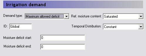
6.1 Demand Type
User Specified
For the User Specified demand type, the demand is not calculated. Rather it is simply specified as a constant value or as a time series.
Crop stress factor
The crop stress factor is the minimum allowed fraction of the crop specific reference ET that the actual ET is allowed to drop to before irrigation starts . That is, the minimum allowed is \((Actual ET)/(Reference ET x K_c* relationship\). This should be a value between 1 and 0. If the actual Crop Stress factor falls below the given value, irrigation will be added.
Ponding depth
When using this option, the demand will be equal to the difference between the actual ponding depth and specified ponding depth. The option is typically used for modelling irrigation of paddy rice. If the ponding depth falls below the specified value then more irrigation water is added.
Max allowed deficit
The available water for crop transpiration (AW) is the difference between the actual water content and the water content at the wilting point for the root zone. The maximum available water for crop transpiration (MAW) is then the value of AW for the reference moisture content, where either the saturated water content or the field capacity can be specified for the reference moisture content. The deficit can then be defined as the fraction of the MAW that is missing and is a value between 0 and 1, where 0 is the deficit when the actual moisture content is equal to the reference moisture content, and 1 is the deficit when the available water for crop transpiration is zero, which is when the water content drops below the water content at the wilting point. When using the Max Allowed Deficit method, irrigation is started when the deficit exceeds the moisture deficit start value and stops at the moisture deficit end value.
If, for example, the reference moisture content is the field capacity and irrigation should start when 60 % of the maximum available water in the root zone is used and cease when field capacity is reached again, the value for the Start should be 0.6, and the value for the Stop value should be 0
6.2 Reference Moisture Content
If the Maximum allowed deficit is used, then the reference moisture content can be either for calculating the deficit is either the saturated water content or the field capacity water content.
6.3 Temporal Distribution
In each of the demand types the demand factor can be specified as a constant value or as a time series. However, an additional option in this combobox is to use the Vegetation Properties file. To use this option, you must include a vegetation properties file when you specify the vegetation. Further, you must specify the irrigation properties in the vegetation properties file itself. In this case, the Vegetation properties file, will contain all of the values needed by each of the different methods and the demand values cannot be input in this dialogue.
7. Irrigation Priorities
| Parameter | Description |
|---|---|
| Conditions | Irrigation selected in Land Use and UZ and ET simulated and Priorities option selected in Land Use dialogue |
| dialogue Type | Integer Grid Codes |
| EUM Data Units | Grid Code |
If there is insufficient water available to satisfy all of the irrigation demand, then the irrigation areas can be prioritised. In this case, each area of the model can be assigned a priority number (1 = highest priority). All the areas with the highest priority will be irrigated first. If there is sufficient water after the first areas have been irrigated, then the areas with the next highest priority will be irrigated.
However, if there is insufficient water to completely satisfy the demand of a particular priority region (all of the cells with priority value = 1, for example), then the water will be distributed to each of the cells based on either Equal Volume or Equal Shortage. The choice of the two priority schemes is assigned in the main Land Use dialogue.
Equal Volume - If the water is to be distributed based on equal volume, then all cells with the same priority number will receive an equal amount of water, regardless of their actual demand. For example, if there is a demand for 100 m3 of water in 10 cells, but only 50 m3 is available, then each cell will receive 5 m3 of water, regardless of the actual demand.
Equal Shortage - If the water is to be distributed based on equal shortage, then all cells with the same priority number will receive an amount of water that satisfies an equal percentage of their actual demand. For example, if there is a demand for 100 m3 of water in 10 cells, but only 50 m3 is available, and 5 of the cells have a demand of 15 m3, while 5 have a demand of only 5 m3, then the first cells will receive 7.5 m3, while the latter will receive only 2.5 m3.
8. Irrigation Log Areas
| Parameter | Description |
|---|---|
| Conditions | Irrigation selected in Land Use and UZ and ET simulated and Priorities option selected in Land Use dialogue |
| dialogue Type | Integer Grid Codes |
| EUM Data Units | Grid Code |
For each of the specified areas one time series file (.dfs0) will be created summarising the simulated irrigation. Note that there is a technical limit to the number of dfs files that can be written.