Reactive Transport
Several reaction processes can be added to the solute transport calculations including
- Sorption and desorption,
- Degradation, and
- Plant uptake.
In the saturated and unsaturated all three of these processes are available. However, in the overland flow only degradation is available, but in MIKE 1D advanced reactions are possible using MIKE ECO Lab, which is a general equation solver for any kinetic reaction process.
The conservative transport of solutes in the unsaturated zone and in the groundwater is governed by the normal advection-dispersion equation described in Equation (36.3). When processes, such as sorption and decay, are included, the equation is extended to
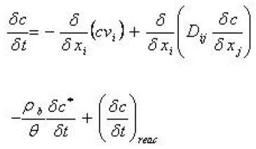
Equation 37.01
where - \(\rho_b\) is the bulk density of the porous medium - \(\theta\) is the porosity of the porous medium - \(c \star\) is the mass of solutes sorbed per dry unit weight of solid - the term \(\delta c/ \delta t\) on the right hand side is a term indicating a biological or chemical reaction of the solute.
This way of describing reaction processes is very simplified and, in some cases, may give incorrect results. Nevertheless, it is a very common way of describing the reaction processes in hydrologic systems.
1. Sorption
Sorption includes a number of geochemical and chemical reactions, such as adsorption of solutes to the aquifer material surface by electrostatic forces (called cation exchange). If these processes occur sufficiently fast compared with the water flow velocity they can be described by an equilibrium sorption isotherm.
Different equilibrium sorption isotherms have been identified from experimental results with different sediments, soils and rock types, see, for example, Fetter, 1992. MIKE SHE AD includes three of the most commonly applied isotherms - namely the linear, Freundlich and Langmuir equilibrium sorption isotherms.
Sorption processes that are slow compared with the water flow velocity must be described by a kinetic sorption isotherm. In MIKE SHE AD the three equilibrium sorption isotherms have been extended to include a kinetically controlled sorption process so that a certain part of the sorbed matter is “transferred” to another part of the soil material.
a. Equilibrium Sorption Isotherms
The linear sorption isotherm is mathematically the simplest isotherm and can be described as a linear relationship between the amount of solute sorbed onto the soil material and the aqueous concentration of the solute:
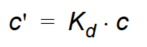
Equation 37.02
where - \(K_d\) is known as the distribution coefficient.
The distribution coefficient is often related to the organic matter content of the soil by an experimentally determined parameter (\(K_{oc}\)) which can be used to calculate the \(K_d\) values.
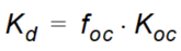
Equation 37.03
where - \(f_{oc}\) is the fraction of organic carbon.
The retardation factor, \(R\), is the ratio between the average water flow velocity (\(v\)) and the average velocity of the solute plume (\(v_c\)). The retardation factor is calculated as
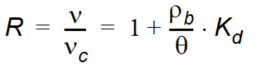
Equation 37.04
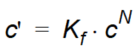
The Freundlich sorption isotherm is a more general equilibrium isotherm, which can describe a non-linear relationship between the amount of solute sorbed onto the soil material and the aqueous concentration of the solute:
Equation 37.05
where - \(K_f\) and \(N\) are constants. Note that the units of Kf is a function of the units of c.
The relationship between K and N is shown in Figure 37.1.
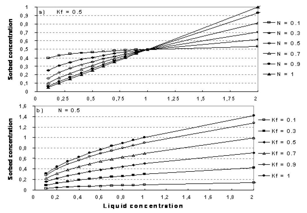
Figure 37.1 Illustration of the Freundlich isotherm. a) effect of change in N, b) effect of change in Kf
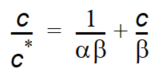
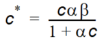
Both the linear and the Freundlich isotherm suffer from the same fundamental problem. That is, there is no upper limit to the amount of solute that can be sorbed. In natural systems, there is a finite number of sorption sites on the soil material and, consequently, an upper limit on the amount of solute that can be sorbed.The Langmuir sorption isotherm takes this into account. When all sorption sites are filled, sorption ceases. The Langmuir isotherm is often given as
Equation 37.06
Equation 37.07
where - \(\alpha\) is a sorption constant related to the binding energy - \(\beta\) is the maximum amount of solute that can be absorbed by the soil material.
The relationship between \(\alpha\) and \(\beta\) is shown in Figure 37.2.
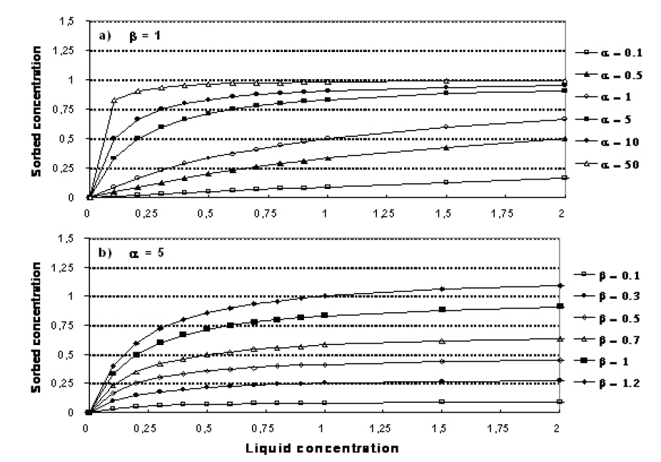
Figure 37.2 Illustration of the Langmuir isotherm. a) effect of change in \(\alpha\), b) effect of change in \(\beta\).
b. Kinetic Sorption Isotherms
The three equilibrium sorption isotherms described so far can be extended to include kinetically controlled sorption. In the MIKE SHE AD module, a two-domain approach is used, where the sorption is assumed to be instantaneous for a fraction of the sorbed solute and rate-controlled for the remainder. A chemical formulation of this approach is given by:
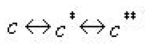
Equation 37.08
where - \(c \star\) is the amount of the solutes sorbed (described by the equilibrium sorption model) - \(c\star \star\) is the amount of the sorbed matter that is converted to the kinetically controlled sorption domain. Mathematically the work of Brusseau (1995) is implemented in MIKE SHE AD as
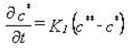
Equation 37.09
where - \(K_1\) is the constant defining the rate of kinetic sorption. The formula is generalised so that effects of hysteresis can be taken into account, by specifying a \(K_1\) value for adsorption (\(c>c \star \star\)) and another value for desorption (\(c\star \star>c \star\)).
The formula is generally applicable for all the equilibrium sorption models. All constants appearing in the sorption models are assumed constant in time but may vary in space.
c. Sorption in Dual Porosity Systems
Sorption depends on the porosity and the bulk density of the soil. In dual porosity systems this is rather complicated. The distribution of sorption between the matrix and the fractures should be calculated based on the bulk density and different porosities. However, this is not always practically possible, so MIKE SHE has included a ‘sorption bias factor', \(F_b\). This allows you to explicitly control the sorption distribution between the fractures and the matrix.
Mathematically, the bulk mass available for sorption in the macro pores, \(\rho_{ma}\), is described by:
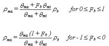
Equation 37.10
where - \(F_b\) is the sorption bias factor - \(\rho_b\) is the bulk mass - \(\theta_{ma}\) and \(\theta_{mi}\) are the macro pore and the matrix porosity respectively. The available bulk mass for sorption in the macropores is “the remainder” mass in the soil. If \(F_b=0\) the distribution of sorption sites between macro pores and matrix is assumed to be proportional to the distribution of porosities. If \(F_b=1\) sorption is assumed to occur in macro pores only and if \(F_b=-1\) sorption is only occurring in the matrix region. The nature of Eq. (37.10) is illustrated in Figure 37.3.
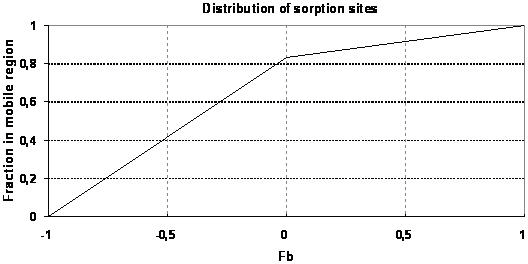
Figure 37.3 Illustration of the fraction of sorption sites located in the macro pore region (\(\rho_{ma}/\rho_b\)) as a function of \(F_b\). \(Mobile porosity = 0.25\), \(immobile porosity=0.05\).
2. Decay
Biological degradation, radioactive decay or other kinds of attenuation of solutes can often be described as a first-order degradation process, with an exponential decrease of concentration over a half-life. This is described in MIKE SHE as
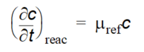
Equation 37.11
where - \(\mu_{ref}\) is the reference degradation rate coefficient calculated by
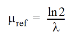
Equation 37.12
where - \(\lambda\) is the half-life of the species.
Following the work of Boesten and van der Linden (1991), to overcome some of the difficulties in simplifying complex biological and chemical reactions, the decay in MIKE SHE is dependent of the soil moisture content and soil temperature as
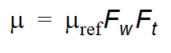
Equation 37.13
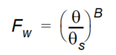
where - the \(F_w\) is the water content function given as
Equation 37.14
and where - \(\theta\) is actual soil moisture - \(\theta_s\) is saturated moisture content - \(B\) is an empirical constant.
\(Ft\) is the soil temperature function given as:

Equation 37.15

Equation 37.16

Equation 37.17
where - \(T_s\) is the actual temperature of the soil - \(T_{ref}\) is the reference temperature at which \(\mu_{ref}\) is measured - \(\alpha\) is a constant depending on \(T\), \(T_{ref}\), the gas constant and the molar activation.
For simplicity the soil temperature over depth is calculated as a function of the air temperature by an experimentally derived formula given by Klein (1995)

Equation 37.18
where - \(T_{sy}\) is the mean daily soil temperature from yesterday - \(T_{air}\) is the mean daily air temperature - \(z\) is depth
Note that for large depths, this function responds very slowly to variations in air temperature. Therefore, long simulations may be necessary to achieve the required initial temperature distribution. An example of simulated soil temperature distributions as a function soil depth is shown in Figure 37.4.
MIKE SHE allows you to specify separate half-lives for the matrix and fractions in dual porosity models, since degradation is likely to be faster in the fractures where higher oxygen contents are more likely.
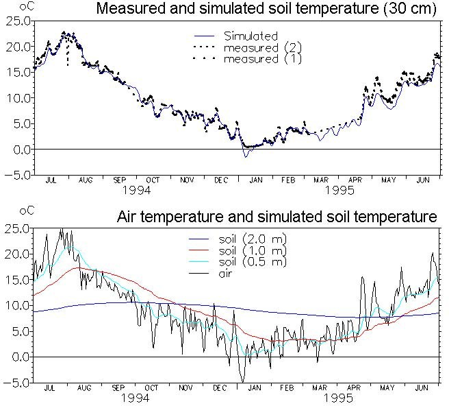
Figure 37.4 Application of the soil temperature function. Top: measured and simulated soil temperature in 30 cm depth (measurements were based on two replicates). Bottom: soil temperatures simulated in different depths based on measured air temperatures.
3. Plant Uptake
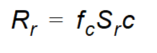
Plant uptake of solutes is described as passive transport, along with the transpiration stream as a function of the solute concentration in the liquid phase. Different roots have different capabilities when it comes to filtering out various solutes. Thus, an empirical concentration factor determines to what extent the available solute is taken up by the plants.
Equation 37.19
where - \(R_r\) is the sink term in the advection-dispersion equation - \(f_c\) is the concentration factor - \(S_r\) is the root water uptake - \(c\) is the liquid concentration.
4. Process verification
a. Overview
The performance of MIKE SHE’s basic reactive transport module, with equilibrium and non-equilibrium sorption and degradation, has been verified against analytical solutions calculated with CXTFIT (Toride et al., 1995). The verification tests were conducted using steady-state saturated water flow through a 1 m deep column discretised in 5 cm elements. The simulations were run for one month with maximum time step equal to 15 min. Pore flow velocity was 25 cm/day, the dispersivity was 1 cm and the bulk density was 1.5 g/cm3. Furthermore, the diffusion process in fractured media with a fracture porosity of 0.25 and a matrix porosity of 0.05 is verified both without and with sorption.
The verification results confirm that the numerical solutions are satisfactory, since the calculated solute breakthrough and mass recovery curves are very similar to the analytical solutions.
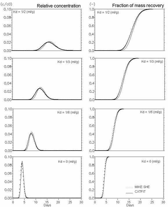
Figure 37.5 Linear equilibrium sorption. Effect of \(K_d\) (ml/g)
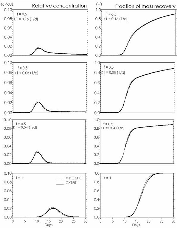
Figure 37.6 Kinetic sorption . Effects of rate constant K1 (\(d^{-1}\)) in Eq.(37.9). Input to CXTFIT: f (fraction of equilibrium sorption sites). \(K_d = 0.5 ml/g\). Input to MIKE SHE: \(Kd = f \cdot K_d (CXTFIT)\). At \(f=1\) the function is reduced to equilibrium sorption with \(K_d = 0.5 ml/g\).
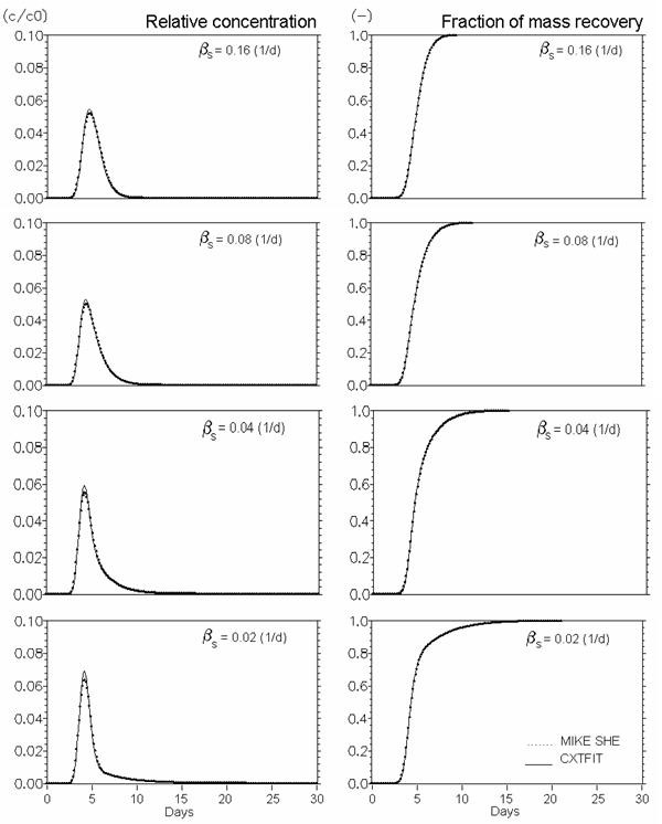
Figure 37.7 Conservative solute transport in dual porosity systems. \(Mobile porosity = 0.25\), \(immobile porosity = 0.05\). Effect of mass transfer coefficient (\(\beta_s\) in Eq. (36.16) (\(d^{-1}\))).
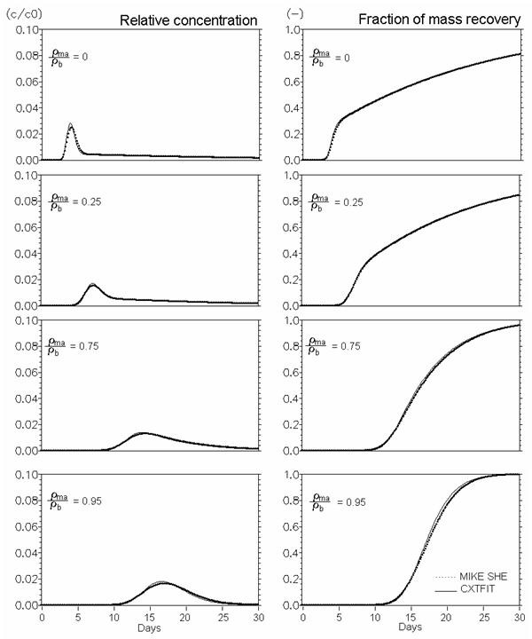
Figure 37.8 Verification of reactive solute transport in dual porosity systems. \(Mobile porosity = 0.25\), \(immobile porosity = 0.05\). Effect of distribution of sorption sites between mobile and immobile regions (\(\rho_{ma}/\rho_b\) Eq. 47) (\(Kd = 0.5 ml/g\), mass transfer coefficient (\(\beta_s\)) = 0.08 \(d^{-1}\)).
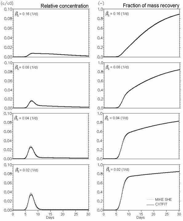
Figure 37.9 Verification of reactive solute transport in dual porosity systems. \(Mobile porosity = 0.25\), \(immobile porosity = 0.05\). Effect of mass transfer coefficient (\(\beta_s\) in Eq. (36.16) (\(d^{-1}\))). \(Kd = 0.5 ml/g\), and \(\rho_{ma}/\rho_b = 0.25\) (Eq. 37.10).
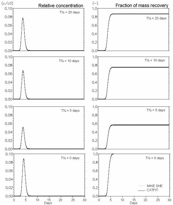
Figure 37.10 Verification of the description of first order degradation. Effect of half life time - T½ (\(\Lambda\)) (days) (Eq. (37.12).
b. Other Processes - Simulation Examples
Some of the process descriptions included in MIKE SHE are too complex to be verified against analytical solutions, including transport of “reactive” solutes in the unsaturated zone under different soil hydrological conditions, plant uptake of solutes, transport in macropores in the unsaturated zone and the influence of temperature and soil moisture content on degradation processes.
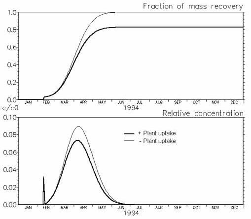
To illustrate one of these cases, plant uptake of solutes is simulated in Figure 37.11. If plant uptake is included a “concentration factor” (see Eq. (37.19)is needed, indicating to which extent solutes are taken up by the plants.
Figure 37.11 Illustration of the effect of plant uptake on solute breakthrough. Plant uptake was simulated with \(fc = 0.5\). The early peak concentrations arise from macro pore transport and were almost alike in the two simulations.