Simulation Specification
1. Introduction
a. Overview
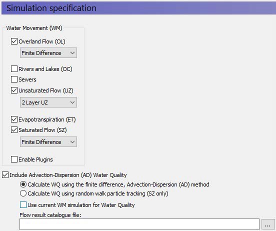
The Simulation Specification dialogue is the key dialogue in the program. In this dialogue, you can select the key options for each of the components included in the simulation, including:
- Overland Flow - see Overland Flow - Technical Reference)
- Rivers and Lakes - see Channel Flow - Technical Reference
- Unsaturated Flow - see Unsaturated Zone - Technical Reference
- 1DRichards Equation
- simplified 1D Gravity Flow
- Two-Layer Water Balance for shallow water tables
- Evapotranspiration - see Evapotranspiration - Technical Reference
- Saturated Flow - see Saturated Flow - Technical Reference)
These choices are immediately reflected in the data tree, where the appropriate parameters are added or removed.
There is only one calculation option in this dialogue for Rivers and Lakes because the calculation methods are defined in the MIKE+ User Interface. Likewise, the use of the simple or advanced Evapotranspiration methods are defined by the unsaturated flow method selected.
b. Water Quality options
Include Advection Dispersion (AD) Water Quality
At the bottom of this dialogue is a checkbox, where you can specify whether or not to include water quality in the simulation. If checked, the data tree will expand to include water quality data items.
PT versus AD
Below the initial checkbox to include water quality, there is a radio button to select the water quality method. There are two methods for calculating water quality in MIKE SHE.
The traditional Advection dispersion method can be used to calculate the movement of multiple solutes throughout the hydrologic system, including sorption and degradation.
The particle tracking (PT) method tracks the movement of thousands of particles that move with the water. The PT method is currently only available in the saturated zone. The PT method allows you to calculate well field capture zones and areas of influence.
Use Current WM simulation for Water Quality
If you uncheck this check box, then you will be able to specify a different water movement simulation as the source of the cell-by-cell flows for the water quality simulation. This allows you to use one water quality setup and calculate water quality based on several water movement scenarios. You must be careful though to not overwrite your results files from the previous water quality simulations.
c. Related Items:
- Working with Solute Transport - User Guide
- Particle Tracking-Reference
- Advection Dispersion - Reference
2. Simulation Title
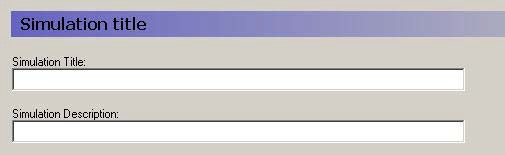
Title and Description The Title and Description will be written to output files and appear on plots of the simulation results.
3. Simulation Period
a. Overview:
In the MIKE SHE GUI, all of the simulation output is in terms of real dates, which makes it easy to coordinate the input data (e.g. pumping rates), the simulation results (e.g. calculated heads) and field observations (e.g. measured water levels).
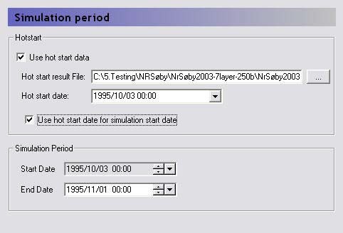
The Simulation Period dialogue is primarily used to define the beginning and end of a transient simulation or the beginning and end of the averaging period for a steady-state simulation.
However, the simulation can be started from a hot start file. A hot start file is useful for simulations requiring a long warm up period or for generating initial conditions for scenario analysis. To start a model from a previous model run, you must first save the hot start data, in the Storing of Results dialogue.
Hot start date The hot start information is saved at specified intervals, and the list of hot start dates is automatically filled in from the hot start file.
Use Hot start date for simulation start date If you select this option, the simulation start date is greyed out and the simulation starts from the selected hot start date. Otherwise, you are free to choose an independent starting date and only the hot start data is simply used as initial conditions.
b. Related Items:
4. Time Step Control
a. Overview
| Time Step Control | |
|---|---|
| Conditions | Maximum OL, UZ, and SZ time steps are only active when the component is selected |
Table 11.1
| Variable | Dimensions |
|---|---|
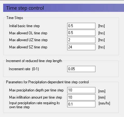
| Initial basic time step | [hrs] |
| Max allowed OL time step | [hrs] |
| Max allowed UZ time step | [hrs] |
| Max allowed SZ time step | [hrs] |
| Increment rate | - |
| Max precipitation depth per time step | [mm] |
| Max infiltration amount per time step | [mm] |
| Input precipitation rate requiring its own time step | [mm/hr] |
b. Time Steps
Initial basic time step This is the initial time step for the Basic time step, unless the component’s maximum allowed time step is less than the initial basic time step. The Basic time step is the “heartbeat” so to speak of the simulation. If all the components are included, this is the UZ time step. If UZ is omitted, then it is the SZ time step. If only OL is included, then it is the OL time step. Assuming all components are included, then one SZ time step can have several Basic time steps, and one Basic time step can include several OL time steps. If the Basic time step changes, for example due to precipitation (see below), then the OL, UZ and SZ time steps change together to maintain their relative sizes.
Max allowed time steps Each of the main hydrologic components in MIKE SHE run with independent time steps. Although, the time step control is automatically controlled, whenever possible, MIKE SHE will run with the maximum allowed time steps. The component time steps are independent, but they must meet to exchange flows, which leads to some restrictions on the specification of the maximum allowed time steps. - If the river model is running with a constant time step, then the Max allowed Overland (OL) time step must be a multiple of the river constant time step. If the river model is running with a variable time step, then the actual OL time step will be truncated to match up with the nearest river time step. - The Max allowed UZ time step must be an even multiple of the Max allowed OL time step, and - The Max allowed SZ time step must be an even multiple of the Max allowed UZ time step.
Thus, the overland time step is always less than or equal to the UZ time step and the UZ time step is always less than or equal to the SZ time step.
If you are using the implicit solver for overland flow, then a maximum OL time step equal to the UZ time step often works. However, if you are using the explicit solver for overland flow, then a much smaller maximum time step is necessary, such as the default value of 0.5 hours.
If the unsaturated zone is included in your simulation and you are using the Richards equation or Gravity Flow methods, then the maximum UZ time step is typically around 2 hours. Otherwise, a maximum time step equal to the SZ time step often works.
Groundwater levels react much slower than the other flow components. So, a maximum SZ time step of 24 or 48 hours is typical, unless your model is a local-scale model with rapid groundwater-surface water reactions.
c. Increment of reduced time step length
Increment rate This is a factor for both decreasing the time step length and increasing the time step length back up to the maximum time step, after the time step has been reduced. See Parameters for Precipitation-dependent time step control for more details on when and how the time step is changed. A typical increment rate is about 0.05.
d. Parameters for Precipitation-dependent time step control
Periods of heavy rainfall can lead to numerical instabilities if the time step is too long. To reduce the numerical instabilities, a time step control has been introduced on the precipitation and infiltration components. You will notice the effect of these factor during the simulation by suddenly seeing very small-time steps during storm events. If your model does not include the unsaturated zone, or if you are using the 2-Layer water balance method, then you can set these conditions up by a factor of 10 or more. However, if you are using the Richards equation method, then you may have to reduce these factors to achieve a stable solution.
Max precipitation depth per time step If the total amount of precipitation [mm] in the current time step exceeds this amount, the time step will be reduced by the increment rate. Then the precipitation time series will be re-sampled to see if the max precipitation depth criteria has been met. If it has not been met, the process will be repeated with progressively smaller time steps until the precipitation criteria is satisfied. Multiple sampling is important in the case where the precipitation time series is more detailed than the time step length. However, the criteria can lead to very short time steps during short term high intensity events. For example, if your model is running with maximum time steps of say 6 hours, but your precipitation time series is one hour, a high intensity one hour event could lead to time steps of a few minutes during that one-hour event.
Max infiltration amount per time step If the total amount of infiltration due to ponded water [mm] in the current time step exceeds this amount, the time step will be reduced by the increment rate. Then the infiltration will be recalculated. If the infiltration criterion is still not met, the infiltration will be recalculated with progressively smaller time steps until the infiltration criteria is satisfied.
This calculation depends on the amount of ponded water available for infiltration. This is the sum of the ponded water from the previous time step, the rainfall in the current time step and the total irrigation added in the current time step - plus the potential snow melt. The potential snow melt is more difficult because it depends on the air temperature and the wet snow storage fraction. If the air temperature is above the threshold melting temperature and the wet snow storage is greater than 95% of the maximum wet snow storage fraction, then the potential snow release equals the total snow storage.
Input precipitation rate requiring its own time step If the precipitation rate [mm/hr] in the precipitation time series is greater than this amount, then the simulation will break at the precipitation time series measurement times. This option is added so that measured short term rainfall events are captured in the model. For example, assume you have hourly rainfall data and 6-hour time steps. If an intense rainfall event lasting for only one hour was observed 3 hours after the start of the time step, then MIKE SHE would automatically break its time stepping into hourly time steps during this event. Thus, instead of a 6-hour time step, your time steps during this period would be: 3 hours, 1 hour, and 2 hours. This can also have an impact on your time stepping, if you have intense rainfall and your precipitation measurements do not coincide with your storing time steps. In this case, you may see occasional small time steps when MIKE SHE catches up with the storing timestep.
If the precipitation is corrected for elevation, then the calculation first loops over all the cells to estimate the maximum time step length. Then it checks the maximum precipitation criteria and adjusts the time step if necessary.
However, normally, the actual time series is read sequentially until the criteria is met, or the end of the time step is reached. However, if the precipitation is corrected for elevation, the time series are not analyses on a cell-by-cell basis. So, there are time series conditions when the maximum precipitation criteria could still be exceeded.
e. Actual time step for the different components
As outlined above the overland time step is always less than or equal to the UZ time step and the UZ time step is always less than or equal to the SZ time step. However, the exchanges are only made at a common time step boundary. This means that if one of the time steps is changed, then all of the time steps must change accordingly. To ensure that the time steps always meet, the initial ratios in the maximum time steps specified in this dialogue are maintained.
After a reduction in time step, the subsequent time step will be increased by Equation 11.05 until the maximum allowed time step is reached.
Equation 11.05
f. Relationship to Storing Time Steps
The Storing Time Step specified in the Detailed WM time series output dialogue, must also match up with maximum time steps. Thus,
- The OL storing time step must be an integer multiple of the Max UZ time step,
- The UZ storing time step must be an integer multiple of the Max UZ time step,
- The SZ storing time step must be an integer multiple of the Max SZ time step,
- The SZ Flow storing time step must be an integer multiple of the Max SZ time step, and
- The Hot start storing time step must be an integer multiple of the maximum of all the storing time steps (usually the SZ Flow storing time step)
For example, if the Maximum allowed SZ time step is 24 hrs, then the SZ Storing Time Step can only be a multiple of 24 hours (i.e. 24, 48, 72 hours, etc.)
5. OL Computational Control Parameters
a. Overview
| Overland Computational Control Parameters | |
|---|---|
| Conditions | if Overland Flow specified in Model Components |
Table 11.2
| Variable | Units |
|---|---|
| Maximum number of iterations Maximum head change per iteration Maximum residual error | - [m] [m/d] |
| Under-relaxation factor | - |
| Maximum courant number | - |
| Threshold water depth for overland flow | [m] |
| Threshold gradient for applying low gradient flow reduction | - |
| Threshold head difference for applying low gradient flow reduction | [m] |
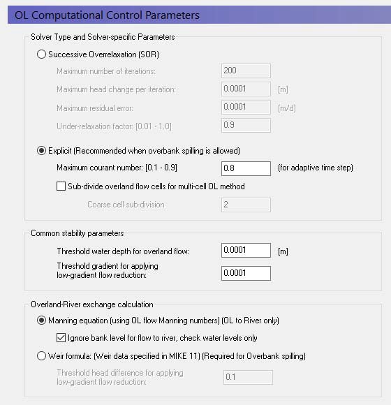
b. Solver Type for Overland Flow
Overland flow can be solved using either using the implicit Successive Over-Relaxation (SOR) Numerical Solution or an Explicit Numerical Solution).
In the SOR method, the depth of overland flow is solved iteratively (implicitly) using a Gauss-Seidel matrix solution. The SOR method is a means of speeding up convergence in the Gauss-Seidel method. The iteration procedure is identical to that used in the saturated zone, except that no over-relaxation is allowed. The SOR method is faster but not as accurate compared to the Explicit method. However, when calculating overland flow to generate runoff, the SOR method is typically accurate enough.
The Explicit method is typically much slower than the implicit SOR method because it usually requires much smaller time steps. However, it is generally more accurate than the SOR method and is often used to calculate surface water flows during flooding. Thus, we recommend that you use the explicit method when overbank spilling from the river to overland flow is allowed.
SOR parameters
Maximum number of iterations If the maximum number of iterations is reached, then simulation will go onto the next time step and a warning will be written to the simulation log file. The default value is 200 iterations, which is normally reasonable. You may want to increase this if you are consistently exceeding the maximum number of iterations, and the residuals are slowly decreasing.
Increasing the following two residual values will make the solution converge sooner, but the solution may not be accurate. However, it may be such that only a couple of points outside your area of interest are dominating the convergence and inaccuracies in these points may be tolerable. Decreasing these values will make the solution more accurate, but the solution may not converge at very small values, and it may take a long time to reach the solution. If you decrease these values, then you may also have to increase the maximum number of iterations.
Maximum head change per iteration If the difference in water level between iterations in any grid cell is greater than this amount, then a new iteration will be started. This will continue until the maximum number of iterations is reached. The default value is 0.0001 m, which is normally reasonable.
Maximum residual error If the difference in water level between iterations divided by the time step length in any grid cell is greater than this amount, then a new iteration will be started. This will continue until the maximum number of iterations is reached. The default value is 0.0001m/d, which is normally reasonable.
Under-relaxation factor The change in head for the next iteration is multiplied by the under-relaxation factor to help prevent numerical oscillations. Thus, lowering the under-relaxation factor is useful when your solution is failing to converge due to oscillations. This will have the effect of reducing the actual head change used in the next iteration. However, often it is more effective to reduce the time step. The under-relaxation factor must be between 0.01 and 1.0. The default value is 0.9, which is normally reasonable.
Explicit parameters
Maximum courant number The courant number represents the ratio of the speed of wave propagation to the grid spacing. In other words, a courant number greater than one would imply that a wave would pass through a grid cell in less than one time step. This would lead to severe numerical instabilities in an explicit solution. The courant number must be greater than 0.1 and less than 1.0. For a detailed discussion of the courant criteria see the Courant criteria.
Subdivide overland flow cells for multi-cell flow method The explicit overland flow solver includes an additional option for solving the water levels on a finer grid scale than the flow velocities. This method also modifies the intercell conductance to account for average flow area across the cell. See Multi-cell Overland Flow Method for more information.
c. Common stability parameters
The common stability parameters are used by both the implicit SOR solver and the explicit solver.
Threshold water depth for overland flow This is the minimum depth of water on the ground surface before overland flow is calculated. Very shallow depths of water will normally lead to numerical instabilities. The default value is 0.0001 m. The threshold depth for overland flow should not be confused with the Detention Storage. The detention storage is related to the amount of water stored in local depression on the ground surface, which must be filled before water can flow laterally to an adjacent cell.
Threshold gradient for applying low gradient flow reduction In flat areas with ponded water, the head gradient between grid cells will be zero or nearly zero and numerical instabilities will be likely. To dampen these numerical instabilities in areas with low lateral gradients a damping function has been implemented. The damping function essentially increases the resistance to flow between cells. This makes the solution more stable and allows for larger time steps. However, the resulting gradients will be artificially high in the affected cells and the solution will begin to diverge from the Mannings solution. At very low gradients this is normally insignificant, but as the gradient increases the differences can become significant. The damping function is controlled by a minimum gradient below which the damping function becomes active. Experience suggests that you can get reasonable results with a minimum gradient between 0.0001 and 0.001. The default minimum gradient is 0.0001. Higher values may lead to a divergence from the Mannings solution. Lower values may lead to more accurate solutions, but at the expense of smaller time steps and longer simulation times. For a detailed discussion of the damping function see the Low gradient damping functionor Threshold gradient for overland flow.
d. Overland River Exchange Calculation
Generally, Overland flow will discharge into the River Link if the water elevation in the cell is higher than the bank elevation of the River Link.
Mannings equation
The rate of discharge to the river is dictated by the Mannings calculation for overland flow. However, this flow is only one way, that is ponded water will flow to the river.
There is a tick box to define the level used to control if flow occurs or not.
- If the tick box is ON, then ponded water will flow to the river if the water level in the cell is above the water level in the River Link (default).
- If the tick box is OFF, then ponded water will flow to the river only if the water level in the cell is above the BANK elevation in the River Link. This was the only option prior to Release 2017. So, to be compatible with older simulations, the tick box must be off.
Weir formula
If you want to include overbank spilling from the river to the overland grid cells, then you must use the weir formula, which provides a mechanism for water to flow back and forth across the riverbank. In this case, the bank is treated like a broad crested weir.
Note
Whether or not to allow overbank spilling from the river to overland flow is set in the river model for each coupling reach. If you do not allow overbank spilling in MIKE+, then the overland river exchange is only one way, but uses the weir formula instead of the Manning’s formula for calculating the amount of exchange flow.
If you do not use the overbank spilling option, then you can still use the flood inundation option to “flood” a flood plain. In this case, though, the flooding is not calculated as part of the overland flow but remains part of the water balance of the river model. For more information on the flood inundation method see the section on Flooding from a MIKE 1D river model to MIKE SHE using Flood codes.
Threshold head difference for applying low gradient flow reduction If the difference in water level between the river and the overland flow cell is less than this threshold, then the flow over the weir is reduced to dampen numerical instabilities. In this case, the same damping function is used as in low gradient areas. The damping function essentially increases the resistance to flow between the cell and the river link. This makes the solution more stable and allows for larger time steps. However, the resulting gradients will be artificially high in the affected cells and the solution will begin to diverge from the Mannings solution. At very low gradients this is normally insignificant, but as the gradient increases the differences can become significant. The damping function is controlled by a minimum head difference between the river and cell below which the damping function become active. Experience suggests that you can get reasonable results with a minimum head difference between 0.05 and 0.1 metres. The default minimum head difference is 0.1. Higher values may lead to a divergence from the Mannings solution. Lower values may lead to more accurate solutions, but at the expense of numerical instabilities, smaller time steps and longer simulation times.
e. Related Items:
- Low gradient damping function
- Overland Flow - Technical Reference
- Working with Overland Flow and Ponding
6. UZ Computational Control Parameters
a. Overview
| UZ Computational Control Parameters | |
|---|---|
| Conditions | if Unsaturated Flow specified in Model Components |
Table 11.3
| Variable | Units |
|---|---|
| Maximum profile water balance error | EUM [water level] |
| Maximum number of iterations | - |
| Iteration Stop criteria | - |
| Maximum water balance error in one node | m |
The unsaturated flow is solved iteratively when the Richards Equation method is chosen but is solved directly for both the Gravity Flow module and the Two-Layer Water Balance methods.
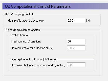
b. UZ-SZ Coupling Control
Since the Two-Layer Water Balance method does not calculate a water table, the UZ-SZ coupling control is only used in the Richards Equation and Gravity Flow modules.
Maximum profile water balance error The tolerance criteria in the UZ-SZ coupling procedure is the maximum allowed accumulated water balance error in one UZ column. If this value is exceeded the location of the groundwater table will be adjusted and additional computations in the UZ component will be done until this criterion is met. The recommended value is 1e-5 m or less. Details on this coupling procedure can be found in Coupling the Unsaturated Zone to the Saturated Zone .
c. Additional Richards Equation Control Parameters
When the Richards Equation method is used, you can specify:
Maximum number of iterations This is the maximum number of iterations that the Richards Equation implicit solver will do before it goes onto the next time step. If the solver has not converged, a message will be written to the log file.
Iteration Stop Criteria The solution is deemed to have converged when the difference in pressure head between iterations for all nodes is less than or equal to the iteration stop criteria. The recommended value is 0.02m or less.
Maximum water balance error in one node This is defined as the fraction of the total saturated volume in the node. The time step will automatically be reduced if the error is exceeded. The recommended value is 0.03 or less. However, smaller values may lead to very short UZ time steps and long run times.
7. SZ Computational Control Parameters
a. Overview
| SZ Computational Control Parameters | |
|---|---|
| Conditions | if Saturated Flow specified in Model Components |
For the saturated zone in MIKE SHE there are two solvers to choose from:
- the pre-conditioned conjugate gradient method, and
- the successive over-relaxation method.
The Successive Over-relaxation solver is the original solver in MIKE SHE and the Pre-conditioned Conjugate Gradient Solver is based on the USGS’s PCG solver for MODFLOW (Hill, 1990).
b. Steady-state vs Transient Simulations
The Solver type controls whether or not the simulation is run as a Steady-state model or not - if you chose the Pre-conditioned Conjugate Gradient- Steady-State option then the simulation will be run in steady-state. Otherwise, the simulation will be run as a transient simulation.
If the SZ simulation is steady-state, then the PCG solver is the only solver available. Although the same options are available for both the steady-state and the transient PCG solvers the optimal parameters or combination of parameters and options is most likely different in the two cases. Thus, the recommended settings are different in both cases.
c. Iteration Control
Table 11.4
| Variable | Units |
|---|---|
| Maximum number of iterations | - |
| Maximum head changed per iteration | The same unit as specified by the EUM [elevation] |
| Maximum residual error | [m/day] |
The iteration procedure can be stopped when either the iteration stop criteria are reached or when the maximum number of iterations is reached. The iteration stops criteria consist of a mass balance criterion and a head criterion. Both of these criteria must be chosen carefully to ensure that the solution has converged to the correct solution.
The default option settings normally perform well in most applications. Usually there is no need for changes. Changes to the default options should not be done unless the solution does not converge, or convergence is extremely slow.
Maximum number of iterations The maximum number of iterations should be sufficiently large to avoid water balance errors due to non-convergence.
Maximum head change per iteration The head criteria determine the accuracy of the solution. The computational time is very dependent on the value used. A value of 0.01m (0.025ft) is usually sufficient. During the initial model calibration, a higher stop criterion can be used. The sensitivity of the head stop criteria should always be examined.
Maximum residual error The maximum residual error is the tolerable mass balance error, which should be low but sufficiently high that the number of iterations is not excessive. A value of 0.001m/d is usually good for regional groundwater studies. In smaller scale applications, where solute transport will be investigated the mass balance criteria should be reduced, for example, to 0.0001 or 0.00001m/d. In general, a larger mass balance criteria should be used during model calibration to keep the initial simulation times shorter. For scenario calculations, the mass balance criteria can be reduced to ensure more accurate simulations and smaller mass balance errors. The SZ water balance should always be checked at the end of the simulation to ensure that the mass balance criteria used was reasonable.
d. Sink de-activation in drying cells
Table 11.5
| Variable | Units |
|---|---|
| Saturated thickness threshold | The same unit as specified by the EUM [water level] (e.g. [ft] or [m]) |
Saturated thickness threshold To avoid numerical stability problems the minimum depth of water in a cell should always be greater than zero. However, if the water depth is close to zero, then sinks in the cell, such as wells, should be turned off, since the cell is effectively ‘dry’. This value is the minimum depth of water in the cell and the depth at which the sinks are deactivated.
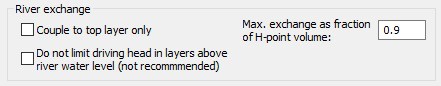
e. River exchange
Table 11.6
| Variable | Units |
|---|---|
| Maximum exchange as fraction of H-point volume | - |
Max. exchange as fraction of H-point volume This represents the maximum amount of water that can be removed from the river during one SZ time step. Removing larger amounts of water could effectively dry out the river. If this occurs, then the SZ solver will issue a warning and only this fraction of water will be removed, which prevents rapid drying out of the river during a single time step.
Couple to top Layer only Calculate groundwater river exchange for the top layer only.
Do not limit driving head in layers above river water level If the river water level drops below the bottom of the layer, the driving head physically does not depend on the river water level. Instead, it is the difference between the head in the layer and the layer bottom. Mainly for backwards compatibility with older models' results this can be switched on so that the full head difference between groundwater and river will be used.
f. Pre-conditioned Conjugate Gradient
Advanced Settings
Gradual activation of SZ drainage To prevent numerical oscillations the drainage constant may be adjusted between 0 and the actual drainage time constant defined in the input for SZ drainage. The option has been found to have a dampening effect when the groundwater table fluctuates around the drainage level between iterations (and does not entail reductions in the drain flow in the final solution). For the steady-state solver and the transient solver the option is by default turned ON.
Horizontal conductance averaging between iterations To prevent potential oscillations of the numerical scheme when rapid changes between dry and wet conditions occur a mean conductance is applied by taking the conductance of the previous (outer) iteration into account. By default, this option is enabled for both steady-state and transient simulations.
Under-relaxation Under-relaxation factors can be calculated automatically as part of the outer iteration loop. The algorithm determines the factors based on the minimum residual-2-norm value found for 4 different factors. To avoid numerical oscillations the factor is determined as 90% of the factor used in the previous iteration and 10% of the current optimal factor. The second option is to define a constant relaxation factor between 0 and 1. In general a low value will provide convergence, but at a low convergence rate - i.e. with many SZ iterations. Higher values increase the convergence rates, but also the risk of non-convergence. As a general rule a value of 0.2 has been found suitable for most setups. The time used for automatic estimation of relaxation factors may be significant compared to subsequently solving the equations and the option is only recommended in steady-state cases. In transient simulations, ’No under-relaxation’ is recommended.
g. Successive Over-relaxation
Table 11.7
| Variable | Dimensions |
|---|---|
| Relaxation Factor | - |
Over-relaxation
Relaxation factor The speed of convergence also depends on the relaxation coefficient. Before you set up your model for a long simulation, you should test the iteration procedure by running a few short simulations with different relaxation coefficients. This coefficient must be between 1.0 and 2.0, with a typical value between 1.3 and 1.6.