Spatial Data
Spatial data includes all model data that can be location dependent, for example precipitation rates and soil parameters.
1. The Grid Editor
The Grid Editor is a generic MIKE Zero grid tool for all MIKE by DHI software. It is the primary means to edit and manipulate gridded data in MIKE SHE.
The Grid Editor was originally developed for the Marine programs MIKE 21 and MIKE 3. However, this often leads to confusion in the node and layer numbering because MIKE 21 and MIKE 3 use a different nodal system because they are based on a node-centred finite difference scheme.
Whereas MIKE SHE is based on a block-centred finite difference scheme.
Node numbering in the Grid Editor
In the Grid Editor (and in MIKE 21 and MIKE 3) the nodes are numbered starting in the lower left from (0,0), whereas in MIKE SHE the nodes are numbered starting in the lower left from (1,1).
Layer numbering in the Grid Editor
In the Grid Editor (and in MIKE 21 and MIKE 3) the layers are numbered starting at the bottom from 0, whereas in MIKE SHE the layers are numbered starting at the top from 1.
2. Gridded Data Types
There are two basic types of spatial data in MIKE SHE - Real and Integer. Real data is generally used to define model parameters, such as hydraulic conductivity. Integer data is generally used to define parameter zones. Thus, model cells with the same integer value can be associated with a time series or other characteristic.
Furthermore, real spatial parameters can be distinguished by whether or not they vary in time. At the moment Integer zones cannot vary with time.
Thus, spatial parameters can be divided into the following:
Stationary Real Parameters
Stationary Real Parameters can vary spatially but do not usually vary during the simulation, such as hydraulic conductivity. If such parameters do vary in time, then you must divide the simulation into time periods and run each time period as a separate simulation, starting each simulation from the end of the previous simulation. This is most easily accomplished using the Hot Start facility, which is found in the Simulation Period dialogue.
The spatial distribution of stationary real parameters is entered using the Stationary Real Data dialogue
Time Varying Real Parameters
Many spatial parameters are time dependent, such as precipitation rate. In this case, both a spatial distribution, as well as a time series for each cell in the model, must be defined. Spatially distributed parameters that also vary in time are entered using the Time-varying Real Data dialogues
3. Integer Grid Codes
Integer Grid Codes are required when Real data varies in time or when model functions, such as soil profiles and paved areas, are assigned to particular zones. Integer Grid Codes are always integer values and do not vary with time.
For information on entering Integer Codes see the Integer Grid Codes section.
The following is an outline of the parameters that require Integer Grid Codes.
Model Domain
Integer Grid Codes are used to define the inactive areas both inside and outside the model domain. Inactive areas outside of the model and the edge of the model are defined in the Model Domain and Grid section, while inactive, subsurface areas inside of the model are defined as Internal boundary conditions.
Component Calculations
Integer Grid Codes are used to delineate such things as paved areas. In this case, the integer code acts like a flag and the calculations that are done are different depending on how the flag is set.
Model Properties
Integer Grid Codes are used to delineate areas with similar properties. In this case, the integer value defines the zone to which the cell belongs. Thus, it defines which set of model properties is to be assigned to the particular cell.
For example, a model may be divided into five zones each with a different soil profile for the unsaturated zone. In this case, the data tree will expand under the model property to include five separate sub-branches, where the soil profile can be defined.
Time Series
Integer Grid Codes are used to define zones for which Real data varies in time. Thus, a time series for a parameter, such as precipitation rate, can be assigned to a model zone. Similarly to the Model Properties above, the model tree will expand under the parameter to include a separate sub-branch for each zone, where the time series file can be defined.
Time Varying Integers
Grid Codes and Integer values do not normally vary with time. If such parameters do vary in time, then you must divide the simulation into time periods and run each time period as a separate simulation, starting each simulation from the end of the previous simulation using the Hot Start options (see Simulation Period).
4. Gridded (.dfs2) Data
If the parameter is defined using gridded data, then the data must be in DHI’s .dfs2 file format.
The easiest way to create the .dfs2 file is to use the  button, which creates a new grid with the proper default values and attribute type. You can then edit this grid in the MIKE Zero Grid Editor, which can be accessed using the
  button.
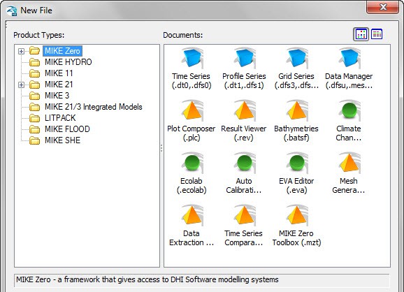
Alternatively, a .dfs2 file can be created using the Grid Series editor, which can be accessed by clicking on File|New in the pull-down menu, or using the New File icon,  , in the toolbar, and then selecting Grid Series.
If you create the file from these tools, you must be careful to ensure that the EUM Data Type matches the parameter that you are creating the file for. For more information on the EUM data types, see EUM Data Units.
The grid for the .dfs2 file does not have to be the same as the numerical model grid. However, if the grids are not subsets of one another then the grids will be interpolated using the bilinear interpolation during the pre-processing stage.
The parameter grid and the model grid are aligned with one another if the parameter grid or the model grid contain an even multiple of the other grid’s cells. For example, if the parameter grid was two times finer, then every model grid cell must contain exactly four parameter grid cells.
If the grids are aligned, then the parameter grid will be averaged to the model grid during the pre-processing stage. However, in some cases it does not make sense to average parameter values. For example, Van Genuchten soil parameters cannot really be averaged, since they are a characteristic of the soil. In such cases, you should ensure that the model grid and the parameter grid file are identical.
Stationary Real Data
Spatially distributed Real parameters, such as conductivity or topography, can be defined in three ways, namely they can be defined as a uniform (global) value or they may be distributed and defined using either gridded data (.dfs2 file), GIS points and polygons (ArcView .shp file), or irregularly distributed point data (x, y, value coordinate file).
It does not make sense to interpolate some parameters to the model grid. In such cases, the use of line and point data should be avoided.
Uniform
A uniform, global value means that all the grid cells in the model will have the same value.
GIS point and line data or Distributed point data
If the parameter is defined using irregularly distributed point data or an ArcView shape (.shp) file, then the data will be interpolated to the model grid during the pre-processing stage, using the interpolation method selected.
The following interpolation methods are included:
It does not make sense to interpolate some parameters to the model grid. In such cases, the use of line and point data should be avoided.
Elevation Data
Elevation data, such as Layer elevations, is handled exactly the same as all other Stationary Real Parameters, except that the value may be optionally specified as a depth below the ground surface rather than absolute elevation above the datum.
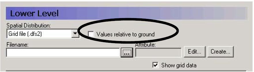
Note
The value must be negative if it is below the ground level.
Tip
The current tools do not allow you to specify a polygon shape file with real values. However, this would be desirable in some cases, such as when implementing Manning’s M values based on vegetation distributions. A trick to get around this limitation is the following:
- Temporarily assign an integer grid code to each of the polygons.
- Specify this file as an input file for one of the data items that needs integer grid codes, such as drain codes.
- Right click on the map that will be displayed and save the map view to a dfs2 file
- Open this dfs2 file in the grid editor and use the grid editor tools to replace the integer values with real values
- In the Grid Editor, change the EUM unit to the appropriate value
- Save the file and then load it into the Data item for which you wanted it.
Time-varying Real Data
If the time-varying Real parameter does not vary spatially then the parameter must be defined as Global with either a Fixed or Time-varying value (see Uniform + Constant and Uniform + Time Varying).
Often, time-varying data, such as precipitation rate, are spatially distributed using measurement stations, which in the model are translated into model zones using, for example, Thiessen polygons. In this case, each station is associated with a .dfs0 time series file that contains the time series of precipitation rate. Sub area-based zones are defined using Integer Grid Codes in either a .dfs2 file as Grid Codes, or in a Shape (.shp) file as polygons with an Integer Code (see Sub area-based + Grid Codes or Polygons).
Uniform + Constant
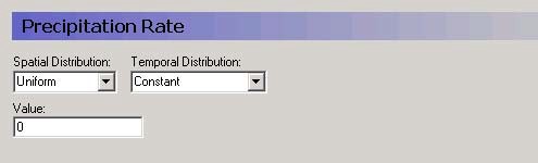
The parameter Value will be assigned to every cell in the model or layer as appropriate and will remain constant throughout the simulation.
Uniform + Time Varying
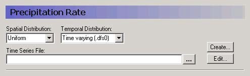
The time series in the .dfs0 file will be assigned to every cell in the model or layer as appropriate.
Sub area-based + Grid Codes or Polygons
Sub area-based time varying data means that the model domain is divided into zones that are defined by an Integer Grid Code.
If a .dfs2 file is used, then the Integer Grid Codes are defined on a regular grid, which is interpreted to the model grid during the Pre-processing stage.
If the Integer Grid Codes are defined using polygons, then you must supply an ArcView .shp file containing polygons each with an Integer Grid Code. The item Fill Gaps with: allows you to define the Integer Grid Code to use in the event that a cell is not included within one of the polygons.
Once the file containing Integer Grid Codes has been defined, a new level in the data tree will appear below the current level, containing one entry for every unique Integer Grid Code in the file.
On this level, you must then supply a time series values for every Integer Grid Code. However, the time series can also be fixed, in the sense that a constant value over time is used. This makes it easy to use detailed time series for some zones and constant values for zones where little information exists.
The time series dialogue itself includes two graphical views. The upper graphic displays the time series that is being applied and the lower graphic shows where the time series will be applied.
Integer Grid Codes
The dialogues for Integer Codes function essentially same as those for Stationary Real Data, except that interpolation does not make sense for integer grid codes.
If Integer Grid Codes are being used to assign Model Properties, such as soil profiles or time series, then new sub-branches will appear in the data tree corresponding to the number of unique Integer Grid Codes in the .dfs2 file.
Uniform Value
A Uniform, global value means that all the grid cells in the model will have the same value. Thus, all cells would belong to the same zone.
Grid File (.dfs2)
If the Integer Code is defined using a grid file, then the Integer Code is defined on a grid. This grid may be different than the numerical model grid. However, the grids must be subsets of one another. That is, the Integer Code grid and the model grid must be aligned with one another and the Integer Code grid or the model grid must contain an even multiple of the other grid’s cells. For example, if the Integer Code grid was two times finer, then every model grid cell must contain exactly four Integer Codes.
Normally, the Integer Code will be assigned to the model grid based on the most prevalent Integer Code in the cell. However, this can lead to problems when a particular code is both infrequent and widely dispersed. For example, if a model area contained many small wetland areas that were much smaller than a grid cell.
For this reason, a bookkeeping count is kept of the assignments to reduce any bias in the assignment of Integer Codes and ensure that less frequently occurring Integer Codes will be represented in the resulting model grid. For example, if there were two different Integer Codes, A and B, used in the model and A always occurred more frequently in each model cell, the bookkeeping count would ensure that B would actually be assigned to some of the model cells. The final frequency of occurrence of the Integer Codes in the model cells would reflect the underlying frequency of occurrence of the Integer Codes. That is, if A occurred twice as often as B, the model grid would also contain twice as many A’s as B’s.
Thus, in our widely dispersed wetland example, if every model grid cell contained 9 Integer Codes for Land Use, and 1/9 of the Land Use grid codes were for wetlands, then every ninth Model Cell would be assigned a Land Use grid code for wetlands.
Polygons
In the current version, only some of the parameters are set up to accept .shp file polygons. Currently, .shp file polygons are only allowed in:
- Model Domain and Grid
- Precipitation Rate
- Vegetation,
- Reference Evapotranspiration
- UZ Soil Profile Definitions,
- SZ Internal boundary conditions, and
- Horizontal Extent of SZ Lenses.
Note
The Horizontal Extent of SZ Lenses accepts polygons, but the dialogue is still set up for point/line .shp files and an error is given in the Data Verification window.
Model grid codes are assigned based in which polygon the centre of the cell is located in.
5. Interpolation Methods
The gap filling is based on the concept that we have to calculate the depth in the point (xc, yc). We define this as the function zc = f(xc, yc). If we place our self in this point, we can divide the world up into four quadrants Q1 - Q4.
From here it’s a matter of finding some points from the raw data set relatively close to this point. The search radius for all possible techniques can be entered - in grid cell distance. Points outside this distance will never be taken into account.
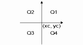
Figure 10.1 Definition of quadrants
Bilinear Interpolation
This technique finds four points from the raw data set - one in each quadrant. The search is done in the following way. A mask of relative indices is created. The cells in this mask are sorted according to the distance. For the quadrant Q1 the cells are sorted in the following way, the grid point itself being excluded.
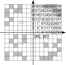
Figure 10.2 Illustration of the neighboring grid cells being sorted
Note that the grid cells with a crosshatch pattern contain raw data points. When the closest raw data point in each quadrant is found, we have four points that form a quadrangle. This quadrangle contains the centre point, where we want to calculate the z-value. This is illustrated on Figure 10.3.
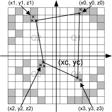
Figure 10.3 Illustration of the closest raw data points in each quadrant.
Note that each grid cell might contain more raw data points. If this is the case, the closest of these is chosen. We now have an irregular quadrangle, where the elevation is defined in each vertex. We need to compute the elevation in (xc, yc). If we transform our quadrangle into a square, we can perform bilinear interpolation. This is illustrated on Figure 10.4)
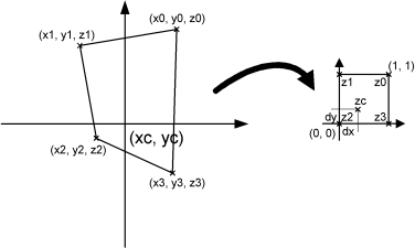
Figure 10.4 Illustration of bilinear interpolation.
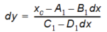
First the interpolation requires the transformation from quadrangle to a normalized square. This is done in the by computing 8 coefficients in the following way:
Equation 10.01
Mapping the coordinates (xc, yc) to the normalized square (dx, dy) is done by solving equation (10.2).
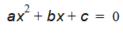
Equation 10.02
where the coefficients are
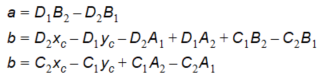
Equation 10.03
Solving equation (10.2) gives us dx.
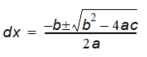
Equation 10.04
where 0 \(\leq\) dx \(\leq\) 1 is used to choose the correct root. dy can now be computed in two ways:
Equation 10.05
Or
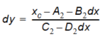
Equation 10.06
Choosing between (10.5) and (10.6) is done in such a way, that division by zero is avoided. (xc, yc) has been mapped to (dx, dy). The task was to compute the elevation in the point (xc, yc) and this is done in the following way using regular bilinear interpolation:

Equation 10.07
If less than four points are found (if one or more quadrants are empty), the double linear interpolation is replaced with reverse distance interpolation (RDI). This is done according to the following scheme:
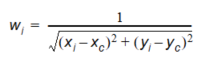
Equation 10.08

Equation 10.09
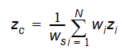
Equation 10.10
The method works fairly efficiently, but it has one drawback. The quadrant search is heavily dependent on the orientation of the bathymetry. If the bathymetry is rotated 45 degrees 4 completely different points might be used for the interpolation. For this reason, there is also a Triangular interpolation method, which can be used, and this method should be direction independent.
Triangular Interpolation
As mentioned previously the ‘Bilinear Interpolation’ is dependent on the orientation of the bathymetry. The ‘Triangular Interpolation’ is made as an answer to this problem. First the closest point to (xc, yc) is found. The following figure shows this:
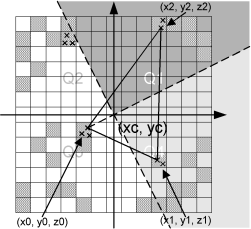
Figure 10.5 Illustration of triangular interpolation
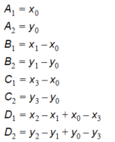
In this example the point (x0, y0, z0) is the closest point. When this point is identified, two quadrants are identified – indicated by the light grey and the dark grey areas. The closest point in these two quadrants are then found. They can be seen on the figure as (x1, y1, z1) and (x2, y2, z2). The interpolation is then done in two steps. First the coefficients describing the plane defined by the 3 found points are computed:
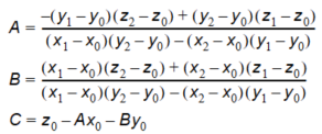
Equation 10.11
And secondly the actual interpolation is done:
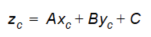
Equation 10.12
If less than 3 points are found, reverse distance interpolation (RDI) is used. The triangular interpolation is more time consuming due to the more complex direction independent search, but better end results should be achieved with this method.
Inverse Distance Interpolation
The two inverse distance interpolation methods both use the nearest point in each quadrant to calculate the interpolated value, weighted by the distance or the distance squared respectively.
6. Performing simple math on multiple grids
In the upper menu of the Grid Editor, under tools, there is an item called Copy File into Data.
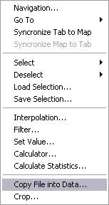
If you select this item, then a dialogue appears where you can insert an existing dfs2 or dfs3 file into the current dfs2 or dfs3 file that you are editing in the Grid editor.
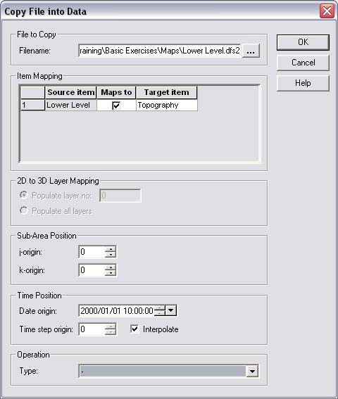
Alternatively, you can define an operation that you want to do with the file. For example, if you were editing a topography file, you could subtract all of the values in a lower elevation file, to obtain a thickness distribution for a layer.
The principal advantage of this tool is that time varying dfs2 and dfs3 files can be manipulated. However, if the operations are complex, but not time varying then
Target file
The target file is the current file you are editing in the Grid editor. The operations that you do are performed on the target file. So, if you don’t want to edit the target file, copy it to a new name first and edit the copy.
File to Copy
The top section of the dialogue is the name of the source file that you want to insert into, subtract from, add to, etc. the target file.
Item mapping
If the target file or the source file has more than one item in it, then all of the items will be listed here, and you will be able to choose whether or not to map the various items to one another.
2D to 3D Layer Mapping
If you are mapping a 2D dfs2 file into a 3D dfs3 file, then you can choose to map all of the layers or only a single layer.
Sub-area position
You select to map the source file onto the target file starting at a different location than the origin. In this case, you must specify the coordinates in the target grid where the origin of the source grid should be positioned. For example, if you have a 20x20 grid and we wish to copy data into the 4x4 rectangle given by the four nodes (10,14), (13,14), (13,17) and (10,17), then you should select a 4x4 grid file and specify j-origin=10 and k-origin=17.
!!!Note: The Grid editor starts its nodal numbering at 0,0.
Time Position
The source grid and target grid do not have to have equal time steps or the same time origin. In this section of the dialogue, you can specify the time at which the source grid should be added to the target grid. In this way, you can add additional time steps to the end of a time varying dfs2 file, or insert hourly information into a monthly time series, for example.
Operation
Finally, you can specify how the source grid file should interact with the target file.
Copy All values are copied such that they replace the existing data in the data set
Copy if target differs from delete value Values in the source file will be copied into the target file, only if the target value is a delete value
Copy if source differs from delete value Values in the source file will be copied into the target file, only if both the source value and the target values are not delete values
Copy if source AND target differs from delete value - values in the source file will be copied into the target file, only if the source value is not a delete value
| Sign | Description |
|---|---|
| + | the source values will be added to the target values |
| - | the source values will be subtracted from the target values |
| * | the source values will be multiplied by the target values |
| / | the source values will be divided by the target values |
7. Performing Complex Operations on Multiple Grids
In the Toolbox, under MIKE SHE/Util, there is a Grid calculator tool, which allows you to perform complex operations on .dfs2 grid files. The only real limitation is that the grid files must have the same grid dimensions. Thus, this tool is much more flexible than the grid operations available in the Grid Editor. With this tool, you can make complex chains of operations, save the setup, and create batch files. You can also run it from a command line, which can save you a lot of time if you are doing the same operation many times, or after each simulation. The Grid Calculator works like a wizard, with Next and Back buttons to move between dialogue