Plugins application example¶

1. Calculation of the reference evapotranspiration¶

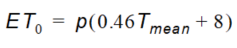
Several methods are available to calculate the reference crop evapotranspiration, depending on the data available. One of these methods is the Blaney- Criddle equation from Brouwer and Heibloem (1986):

Equation 15.01

where

\(ET_0\) is the reference evapotranspiration as an average of a period of one month [mm/day]
\(p\) is the mean daily percentage of annual daytimehours
\(T_{mean}\) is the daily mean air temperature [C].

The following Python plugin calculates the reference evapotranspiration for a 1-year MIKE SHE simulation using the Blaney-Criddle method accordingly to the example provided by Brouwer and Heibloem (1986).

The plugin is composed of three parts:

Importing MShePy module
Creating global variables (P, T_max, and T_min)
Calculating and assigning the evapotranspiration at the beginning of each time step

In order to calculate the evapotranspiration (point 3), the evapotranspiration object is created. Since the temperature and the percentage of daytime hours is given in monthly average, the month of the current time step is used to select the corresponding values for the month. These values are used to calculate the reference evapotranspiration value and assign it to the MIKE SHE simulation. For this example, the evapotranspiration value was chosen to be a global value for the whole model domain.

import MShePy # import the MShePy module
# define global variables
# monthly average of percentage of daytime hours
P = [0.26, 0.26, 0.27, 0.28, 0.29, 0.29, 0.29, 0.28, 0.28, 0.27, 0.26, 0.25]

# monthly average of daily maximum temperature
T_max = [32.1, 35.8, 38, 38.7, 39, 36.6, 32.6, 30.8, 31.8, 34.8, 35, 32]

# monthly average of daily minimum temperature
T_min = [15.5, 18.8, 21.8, 24.5, 26, 25, 22.7, 22, 23, 21.3, 18.7, 16.6]

def preTimeStep(): 
  '''
  Plugin function executed at the beginning of each time step
  '''
  PET = MShePy.dataset(MShePy.paramTypes.ET_REF_EXC) # Create PET dataset
  time = MShePy.wm.currentTime() # Get current simulation time
  month = time.month # current simulation month
  T_mean = (T_max[month-1] + T_min[month-1]) / 2 # Average temperature
  ET = P[month-1] * (0.46 * T_mean + 8) # Calculate ET (mm/d)
  PET.value(ET) # Assign value to PET dataset
  MShePy.wm.setValues(PET) # Set ET values to engine

2. Reference evapotranspiration adjusted for the altitude¶

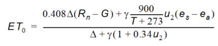
The reference evapotranspiration can be calculated using the modified version of the Penman-Monteith equation presented by Allen et al. (1998):

Equation 15.02

where

\(ET_0\) is the refence evapotranspiration [mm/day]
\(R_n\) is the net radiation at the crop surface [MJ/\(m^2\)/day]
\(G\) is the soil heat flux density [MJ/\(m^2\)/day]
\(T\) is the mean daily air temperature at a 2 m height [°C]
\(u_2\) is the wind speed at a 2 m height [m/s]
\(e_s\) is the saturation vapor pressure [kPa]
\(e_a\) is the actual vapor pressure [kPa]
\(\Delta\) is the slope vapor pressure curve [kPa/°C]
\(\gamma\) is the psychrometric constant [kPa/°C]

This plugin example considers the changes in pressure and, thus, on the psychrometric constant due to the elevation

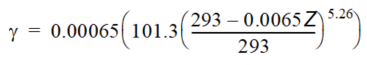
Equation 15.03

where - \(Z\) is the ground elevation [m].

The plugin below reproduces example 17 by Allen et al. (1998). It consists of three parts:

Importing MShePy module
Creating global variables
Calculating and assigning the evapotranspiration at the end of the initialization

The calculation of the \(\gamma\) and, thus, of the evapotranspiration depends on the surface elevation. In the plugin example, Gamma (\(\gamma\)) is calculated using Elevation, which is a MShePy dataset for surface elevation. Thus, Gamma is also a MShePy surface elevation dataset, but it contains value of \(\gamma\), whose unit is [kPa/°C] and not [m]. This is also true for the ET variable, which contains the calculated evapotranspiration. This discrepancy is solved by assigning the value of ET to PET, which is a MShePy reference evapotranspiration dataset. It would have not been possible to calculate the values of PET directly from an equation containing the elevation dataset (Elevation), because then PET would have been changed to an elevation dataset.

import MShePy # import the MShePy module 

# define global variables
Delta =  0.246 # Slope vapour pressure curve (*o*C/kPa)
Rn    = 14.33  # Net radiation at the crop surface (MJ/m2/day)
G     =  0.14  # Soil heat flux density (MJ/m2/day)
T     = 30.2   # Monthly average mean temperature (*o*C)
u2    =  2     # Monthly average daily wind speed measured at 2 m (m/s)
Es    =  4.42  # Monthly average daily saturation vapour pressure (kPa)
Ea    =  2.85  # Monthly average daily actual vapour pressure (kPa)

def postEnterSimulator(): 
  '''
  Plugin function executed after initializations, before the simulation begins
  '''
  # Create PET dataset
  (startTime, currentTime, PET) = MShePy.wm.getValues(MShePy.param Types.ET_REF_EXC)
  PET.convert('mm/day') # Convert the unit of the PET dataset

  # Get the elevation from the MIKE SHE model
  (startTime, currentTime, Elevation) = MShePy.wm.getValues(MShePy.paramTypes.DEM_Z)

  # Calculate the psychrometric constant from the elevation (kPa/*o*C)
  Gamma = 0.00065 * 101.3 * ((293 - 0.0065 * Elevation) / 293)**5.26

  # Calculate reference ET (mm/d)
  ET = (0.408 * Delta * (Rn - G) + Gamma * (900 / (T + 273)) * u2 * (EsEa)) / (Delta+Gamma * (1 + 0.34 * u2))
  PET[:] = ET[:] # Assign calculated value to PET dataset
  MShePy.wm.setValues(PET) # Set evapotranspiration values to engine

3. Managing irrigation as function of precipitation in the previous months¶

Periods with dry conditions will typically require more irrigation compared to wet periods. The following plugin describes a simplified method to optimize the irrigation rate based on the precipitation rate of the previous weeks. At the beginning of each time step, the precipitation rate of the previous month, compared to the current simulation time step, is analyzed. For precipitation rates lower than the annual mean precipitation rate, irrigation is applied to the model. When the previous month has been a wet one (precipitation rate higher than the annual mean), then no irrigation is applied. In this plugin, the irrigation rate is applied to the model as part of the precipitation rate. Thus, a new precipitation rate is calculated as the sum of the observed precipitation and calculated irrigation and passed to the MIKE SHE simulation.

import MShePy
Precipitation = [1.3, 0.7, 1.3, 1, 1.3, 2, 1.9, 1.9, 2, 1.6, 2, 1.6] # Monthly average precipitation (mm/d)

P_mean = 1.6 # Annual mean precipitation (mm/d)

def preTimeStep():
  PreIrr = MShePy.dataset(MShePy.paramTypes.P_RATE) # Create Precipitation+irrigation dataset
  time = MShePy.wm.currentTime() # current simulation time
  month = time.month # Current simulation month
  if Precipitation[month-2] < P_mean: # Condition for irrigation 
    Irrigation = P_mean - Precipitation[month-2] 

    # Calculate the irrigation rate (mm/d)
    PreIrr_rate = Precipitation[month-1] + Irrigation # Calculate irrigation + recharge (mm/d)
    PreIrr.value(PreIrr_rate) # Assign irrigation + recharge
    MShePy.wm.setValues(PreIrr)

4. Using the MIKE IO library together with MShePy¶

A pretty common use case is to combine MShePy together with the MIKE IO library. If you do this, please be aware of that is essential to load the MShePy first, before you load MIKE IO. Otherwise you will get an error.

import MShePy
import mikeio