Working with Rivers and Streams

1. Channel Flow - MIKE 1D Overview

MIKE 1D is a comprehensive 1D channel flow modelling engine for simulating rivers and surface water bodies that can be approximated as 1-dimensional flow (as strict 1-Dimensional flow does not occur in nature). Basically, MIKE 1D can be applied anywhere average values of levels, velocities, concentrations etc. at a point are acceptable, including:

• River hydrodynamics
• Structure/reservoir operational control
• Water quality (e.g. wetlands, salinity)
• Sediment transport & morphology
• Flood studies (e.g. mapping, hazard assessment)
• Flood forecasting (on-line, real-time)
• Dam break
• Sediment transport (e.g. Long term morphology)
• River restoration
• Integrated with groundwater and flooding

MIKE 1D plays a critical role in MIKE SHE Both the overland flow and groundwater flow modules are linked directly to MIKE 1D. The MIKE SHE- MIKE 1D coupling enables:

• the one-dimensional simulation of river flows and water levels using the fully dynamic Saint Venant equations.
• the simulation of a wide range of hydraulic control structures, such as weirs, gates and culverts.
• area-inundation modelling, using a simple flood-mapping procedure that is based on simulated river water levels and a digital terrain model.
• dynamic overland flooding flow to and from the river network.
• the full, dynamic coupling of surface and sub-surface flow processes in the river and MIKE SHE.

2. Building a MIKE 1D river model

Integrating a MIKE SHE and a MIKE 1D river model is not very different from establishing a stand-alone MIKE 1D HD river model and a stand-alone MIKE SHE model. A MIKE 1D model can be built in MIKE+ or, using and older version of MIKE software, in MIKE HYDRO River or MIKE 11. If using MIKE+, the setup needs to be converted to the MIKE 1D format .m1dx using the Export function in MIKE+. The .m1dx file can then be specified in MIKE SHE as the river setup. In release 2024, it's still possible to using MIKE 1D setups built using MIKE HYDRO River and MIKE 11 by linking to the .mhydro and .sim11 extensions, respectively. MIKE HYDRO River and MIKE 11 were discontinued after the 2023 release of MIKE software.

In principle, there are three basic set-up steps:

1. Build a stand-alone MIKE 1D HD hydraulic model and make a performance test and, if possible, a rough calibration using prescribed inflow and stage boundaries. If needed, you can specify a default groundwater table (e.g. MIKE SHE’s initial groundwater level) and leakage coefficients for any leakage calculations.
2. Build a stand-alone MIKE SHE model that includes the overland flow component and (optionally) the saturated zone and unsaturated zone components. An SZ drainage boundary can be used to prevent excessive surface flows in low lying areas and the river flood plain.
3. Couple MIKE SHE and MIKE 1D by defining branches (reaches) where the river HD model should interact with MIKE SHE. Modify your MIKE SHE and MIKE 1D models so that they work together properly. For example, by removing the specified groundwater table in MIKE 1D and adjusting your SZ drainage elevations if you used these in Step 2.

In the above scheme, the first step in coupling MIKE 1D to MIKE SHE is to create a normal MIKE 1D HD river model without coupling it with MIKE SHE. In this regard, a few things should be emphasised:

• In a normal 1D river model only the river chainage (dx) is important for the results. Geographic positioning of river branches and cross-sections are only important for the graphical presentation. When interfacing MIKE 1D to MIKE SHE geographic positioning is critical, as MIKE SHE needs information on the river location.
• A reasonably high number of river cross-sections should be included to ensure that the river elevations are reasonably consistent with the surface topographic features.

2.1 MIKE 1D River Model Network Limitations

There are a few features of MIKE 1D that do not relate well to MIKE SHE.

Short branches

In MIKE 1D there is no restriction on how short your branches are. If you are trying to simulate discontinuous lakes or structures on the flood plain, for example. you may have very short branches. However, MIKE SHE does not allow river branches to be shorter than the cell size. Generally, though, short branches are a sign that you should probably reconsider your model conceptualization - or switch to MIKE+, which allows flood plain structures.

Parallel branches

Like short branches, MIKE SHE does not like it when your branches are too close together. If you have parallel branches that are too close together, then the branches may be mapped to the same river link. However, each river link must be mapped to a unique branch. As a rule of thumb, parallel branches should be greater than a cell width apart. However, this is not uniformly true, since the two close parallel branches may map onto opposite sides of a cell, if they are located on either side of a cell mid-point. Thus, you may have unexpected problems, if you change the cell size in a model that was working and you have branches that are closer together than one cell size.

In a dense river network results may also depend on the order the river branches are being processed. Since version 2021 the branches will always be processed in the same order, regardless of sorting in the river model setup. To do the processing in the order of in which they have been specified in the river model GUI instead, use the extra parameter 'disable initial branch sorting (see Order of creating river links).

Long coupling links

MIKE SHE links to MIKE 1D River branches. However, when two branches are connected, water is passed between the branches directly. The link has no physical length or storage itself. If your links are too long, there will be an error in the timing of the flows between the two branches. So, the links should be kept short. MIKE 1D does not have any restrictions on how long the links can be, but MIKE SHE will issue a warning if the links are longer than a cell size. The warning is simply to informing you that there is no possibility for groundwater-surface water exchange in the link.

Long distances between cross sections

MIKE 1D controls the distance between the calculation nodes. The properties at the calculation nodes are linearly interpolated from the available cross-sections. This includes geometric properties such as bank and bottom elevations, marker locations, etc. However, linear interpolation can easily result in inconsistencies between elevations in MIKE SHE and marker elevations in MIKE 1D. If the bank elevation is higher than the topography, then overland flow into the river will be restricted. If the downstream river bottom elevation is higher than the side branch bottom elevation, then MIKE 1D will likely be unstable.

Long distances between calculation nodes

This is not the same as long distances between cross-sections. MIKE 1D manages the water at the q-points directly linked to the river links. MIKE SHE and the river link system automatically interpolates the nearest river link.

However, if the calculation nodes are very far apart or very close together, then the linear interpolation of water volumes between the calculation points may lead to discrepancies in the available water volumes especially if the river links are being used for irrigation or the river is losing water. In this sense, the distance between the calculation nodes, should be similar to the MIKE SHE grid spacing.

2.2 River Cross-sections

Whenever there is a significant change in the bed slope there should, in principle, be a cross-section at that location. If only a few cross-sections are available, it may be sufficient to estimate the cross-section shape based on neighbouring cross-sections and estimate the bank/bed elevation based on the surface topographic information in MIKE SHE or other topographic maps.

Cross-sections vs. time step

However, every cross-section in MIKE 1D is a calculation node. The time step in MIKE 1D is sensitive to the Courant number, which is proportional to the distance between calculation nodes. So, if the cross-sections are close together, then you may experience very short time steps in MIKE 1D.

Thus, if you have very short river model time steps, then you might want to check your river network to make sure you do not have cross-sections that are too close together. This frequently occurs when the cross-sections have been imported. If you do have cross-sections that are too close together, then you can easily eliminate one or more of them, as long as the conveyance of the different cross-sections is roughly the same. In other words, you can eliminate duplicate cross-sections if their Q/H relationships are roughly the same, even though the physical shape of the two cross-sections may appear quite different. This is often the case in braided stream networks, where the location of the main channels may move left or right, but the overall conveyance of the river bed is relatively constant.

Cross-sections versus MIKE SHE topography

In the absence of flooding, ponded water discharges to the river as overland flow. As a general rule, the topography must be higher than or equal to the bank elevation. If the bank elevation is higher than the topography, water will not be able to flow into the river in that cell, but will run laterally along the river until it reaches a place for it to flow into the river. An easy trick to see where this is happening is to run a simulation with no infiltration, ET, or detention storage and set the initial water depth at 1m. Then look at the results to find places were the water is piling up against the river links.

In the pre-processor log file, a table is create that lists all the river links where the bank elevation is different than the topography.of the adjacent cell. The critical river links with bank elevations above the topography are highlighted with the ==> symbol. This list can be surprisingly long because the river link bank elevations are interpolated from the neighbouring cross-sections.

Whereas the topography is already defined. So, frequently the interpolated bank elevations do not line up precisely with the topography.

If overland flow on the flood plain is essentially absent, for example, due to infiltration or evapotranspiration, then these differences are not relevant and there is no need to modify the topography. However, if the overland to river exchange is important then you may have to carefully modify your topography file or your bank elevations so that they are consistent.

Note

In many cases, your topography is from a DEM that is different from your model grid - either because it is a .shp or xyz file, or if it is a different resolution than your model grid. In this case, it may be easier to save the pre-processed topography to a dfs2 file (right click on the topography map in the preprocessed tab). Then modify and use the new dfs2 file as the topography in your model setup. The disadvantage of this, is that if you change your model domain or grid, then you will have to redo your topography modifications.

Note

You can also use one of the Flood code options to automatically modify your topography, if you have wide cross-sections or a detailed DEM of the floodplain. In this case, after you have set up your river model, you can specify a constant grid code for the whole model and let MIKE SHE calculate a modified topography based on the cross-sections or bathymetry. Then save the topography file as above and then use it as the model topography.

3. Coupling of MIKE SHE and a MIKE 1D River Model

The coupling between MIKE 1D and MIKE SHE is made via river links, which are located on the edges that separate adjacent grid cells. The river link network is created by MIKE SHE’s set-up program, based on a user-specified sub-set of the MIKE 1D model, called the coupling reaches. The entire river system is always included in the hydraulic model, but MIKE SHE will only exchange water with the coupling reaches. Figure 26.1 shows part of a MIKE SHE model grid with the MIKE SHE river links, the corresponding MIKE 1D coupling reaches, and the river h-points (points where MIKE 1D calculates the water levels).

The location of each of MIKE SHE river link is determined from the coordinates of the river model points, where the river points include both digitised points and h-points on the specified coupling reaches. Since the MIKE SHE river links are located on the edges between grid cells, the details of the river model geometry can be only partly included in MIKE SHE, depending on the MIKE SHE grid size. The more refined the MIKE SHE grid, the more accurately the river network can be reproduced.

If flooding is not allowed, the river water levels at the h-points are interpolated to the MIKE SHE river links, where the exchange flows from overland flow and the saturated zone are calculated.

If flooding is allowed, via Flood Codes, then the water levels at the river model h-points are interpolated to specified MIKE SHE grid cells to determine if ponded water exists on the cell surface. If ponded water exists, then the unsaturated or saturated exchange flows are calculated based on the ponded water level above the cell.

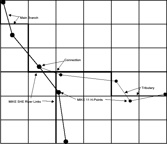
Figure 26.1: MIKE 1D River Branches and h-points in a MIKE SHE Grid with River Links

If flooding is allowed via overbank spilling, then the river water is allowed to spill onto the MIKE SHE model as overland flow.

In each case, the calculated exchange flows are fed back to the river model as lateral inflow or outflow.

Each MIKE SHE river link can only be associated with one coupling reach, which restricts the coupling reaches from being too close together. This can lead to problems when you have a detailed drainage or river network with branches less than one half a cell width apart. It will also lead to problems if your river model branches are shorter than your MIKE SHE cell size.

If you have coupling reaches that are too short or too close together, you will receive an error message. If this happens, you can

• decide not to include one of the branches as a coupling reach (it is still included in the MIKE 1D HD model), or
• remove some of the branches (this error often occurs when you have a detailed looped drainage network), or
• refine your MIKE SHE grid until all coupling reaches are assigned to unique river links.

If you have a regional model with large cells (say 1-2km wide), then you cannot expect the river-aquifer interaction to be accurate at the individual cell level (e.g. all your cell properties – topography, conductivity, Manning’s M, etc. – are all average values over 1-4 km2). Rather, most often you will be interested in having a correct overall water balance along the stream. Typically, this is achieved by calibrating a uniform average river bed leakage coefficient against a measured outflow hydrograph. In such a model, you may also be tolerant of higher groundwater residuals.

On the other hand, if you need more detailed site specific results (and you have data and measurements to calibrate against), then you will use a local scale model, with a smaller grid (say 50-200m) and discrepancies between topography and river bank elevation will largely disappear. In this case, you will be more likely to be able to make accurate local scale predictions of groundwater-surface water exchange.

3.1 MIKE SHE Branches vs. MIKE 1D River Branches

A MIKE 1D branch is a continuous river segment defined in MIKE 1D. A MIKE 1D branch can be sub-divided into several coupling reaches.

A MIKE SHE branch is an unbroken series of coupling reaches of one MIKE 1D branch.

One reason for dividing a MIKE 1D branch into several coupling reaches could be to define different riverbed leakage coefficients for different sections of the river.

If there are gaps between the specified coupling reaches, the sub-division will result in more than one MIKE SHE branch. Gaps of this type are not important to the calculation of the exchange flows between the hydrologic components (e.g. overland to river, or SZ to river). The exchange flows depend on the water level in the river model, which is unaffected by gaps in the coupling reaches.

However, MIKE SHE can calculate how much of the water in the river is from the various hydrologic sources (e.g. fraction from overland flow and SZ exfiltration). However, this sort of calculation is only possible if the MIKE SHE branch is continuous. If there is a gap in a MIKE SHE branch, then the calculated contributions from the different hydrologic sources downstream of the gap will be incorrect. If there are gaps in the MIKE SHE branch network, then the correct contributions from the different sources must be determined from the MIKE 1D output directly.

Furthermore, the MIKE 1D/MIKE SHE coupling for the water quality (AD) module will not work correctly if there are gaps in the MIKE SHE branch network.

There is one further limitation in MIKE SHE. That is, no coupling branch can be located entirely within one grid cell. This limitation is to prevent multiple coupling branches being located within a single grid cell.

Connections Between Tributaries and the Main Branch

Likewise, the connections between the tributaries and the main branch are only important for correctly calculating the downstream hydrologic contributions to the river flow and in the advection-dispersion (AD) simulations. The connections are not important to the calculation of the exchange flows between the hydrologic components (e.g. overland to river, or SZ to river).

In the example shown in Figure 26.1, the river links of the tributary are correctly connected to the main branch. This will happen automatically when

• the hydraulic connection is defined in the MIKE 1D River network, AND
• the connection point (the chainage) on the main branch is included in a coupling reach, AND
• the connection point (the chainage) on the tributary is included in a coupling reach.

If the connection does not satisfy the above criteria, then there may be a gap in the MIKE SHE branch network and the limitations outlined above will apply.

3.2 The River-Link Cross-section

The MIKE 1D (HD) hydraulic model uses the precise cross-sections, as defined in the cross-section file, for calculating the river water levels and the river volumes. However, the exchange of water between the river and MIKE SHE is calculated based on the river-link cross-section.

The river-link uses a simplified, triangular cross-section interpolated (distance weighted) from the two nearest river cross-sections. The top width is equal to the distance between the cross-section’s left and right bank markers. The elevation of the bottom of the triangle equals the lowest depth of the river crosssection (the elevation of Marker 2 in the cross-section). The left and right bank elevations in MIKE 1D (cross-section markers 1 and 3 in the cross section editor) are used to define the left and right bank elevations of the river link (See Figure 26.2).

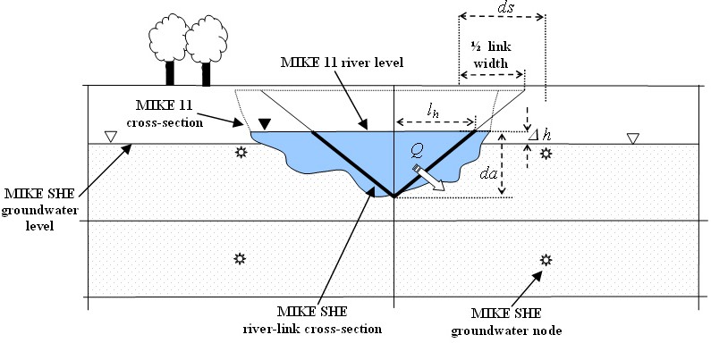
Figure 26.2: A typical simplified MIKE SHE river link cross-section compared to the equivalent MIKE 1D cross-section

If the MIKE 1D river cross-section is wider than the MIKE SHE cell size, then the river-link cross-section is reduced to the cell width.This is a very important limitation, as it embodies the assumption that the river is narrower than the MIKE SHE cell width. If your river is wider than a cell width, and you want to simulate water on the flood plain, then you will need to use either the Flooding from a MIKE 1D river model to MIKE SHE using Flood Codes ]() option or the Direct Overbank Spilling to and from Rivers option.

If you don’t want to simulate flooding, then the reduction of the river link width to the cell width will not likely cause a problem, as MIKE SHE assumes that the primary exchange between the river and the aquifer takes place through the river banks. For more detail on the river aquifer exchange see Groundwater exchange with Rivers.

For more detail on flooding and overland exchange with a river model, see Overland Flow Exchange with Rivers

3.3 Connecting Rivers to MIKE SHE

In MIKE 1D, every node in the river network requires information on the river hydraulics, such as cross-section and roughness factors. These nodes are known as h-points, and MIKE 1D calculates the water level at every H-point (node) in the river network. Halfway between each H-point is a Storing Q-point, where MIKE 1D calculates the flow, which must be constant between the h-points.

The water levels at the river h-points are transferred to the MIKE SHE river links using a 2-point interpolation scheme. That is, the water level in each river link is interpolated from the two nearest h-points (upstream and downstream), calculated from the centre of the link. The interpolation is proportionally distance-weighted.

The volume of water stored in a river link is based on a sharing of the water in the nearest h-points. In Figure 26.3, River Link A includes all the water volume from H-points 1 and 2, plus part of the volume associated with H-point 3. The volume in River Link B is only related to the volume in H-point 3. While the volume in River Link C includes water from h-points 3 and 4. This is done to ensure consistency between the river volumes in MIKE 1D and MIKE SHE, as the amount of water that can infiltrate or be transferred to overland flow is limited by the amount of water stored in the river link.

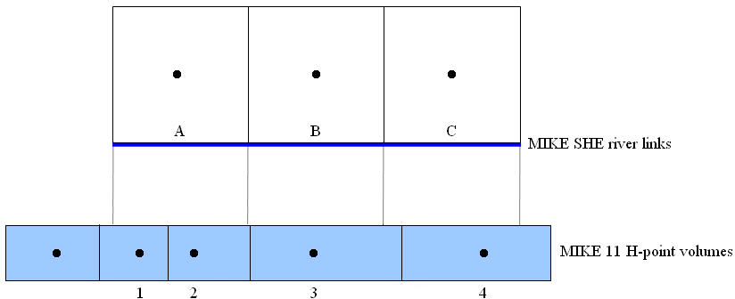
Figure 26.3: Sharing of river model H-point volumes with MIKE SHE river links

The water levels and flows at all river model h-points located within the coupling reaches can be retrieved from the MIKE SHE result file.

However, since the river flows are not used by MIKE SHE, the river flows stored in the MIKE SHE result file are not the flows calculated at the MIKE 1D Q-points. Rather, the flows stored in the MIKE SHE result file are the estimated flows at the h-points. That is, the flows in the MIKE SHE result file have been linearly interpolated from the calculated flows at the Q-point locations to the H-point locations on either side of the Q-point. If the exact Q-point discharges are needed, they must be retrieved or plotted directly from the MIKE 1D result file.

3.4 Evaluating your river links

The river links are evaluated during the pre-processing. In the pre-processor log file (yourprojectnamePP_print.log), there is a table that contains all of the river link details:

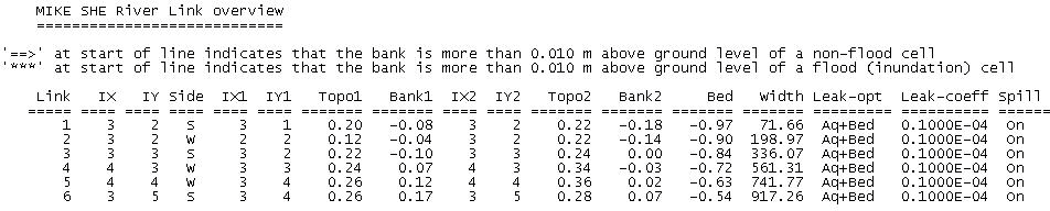
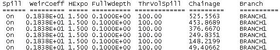
In this table, the locations where the river links are higher than the topography are marked in the outside left column.

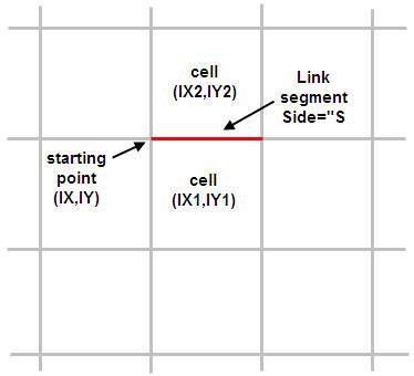
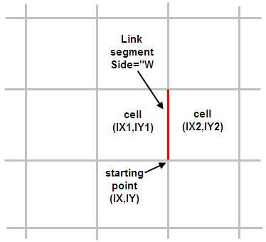
The reference system used in the table is illustrated below:

The explanation of the columns is:

Link: River Link ID number. ID starts at 1 and increases by 1.

IX,IY: coordinate of one end of the link segment. They are referred to the preprocessed grid such that (IX,IY)=(1,1) at the left-bottom corner of the model grid. The link segment can be drawn starting from (IX,IY) coordinate, and then following east direction if Side="S" or following the north direction if Side="W".

Side: relative position of the (IX1,IY1) cell with respect to the link segment. "S" stands for south and "W" for west.

IX1,IY1: coordinate of the cell on the south side of the link if Side="S", or the cell on the west side of the link if Side= "W". The left-bottom corner cell of the model grid has coordinates (IX1,IY1)= (1,1).

Topo1: Pre-processed Topo elevation (in meters) of the cell (IX1,IY1).

Bank1: Interpolated cross section bank elevation (in meters) at marker 1 or 3 at the link chainage (last column). The marker (1 or 3) corresponding to Bank1 depends on the position of the cell (IX1,IY1) with respect to the direction of increasing chainage. Marker 1 is the left marker in the increasing chainage direction.

IX2,IY2: Coordinate of the cell on the opposite side to (IX1,IY1). In other words, it is the cell on the north side of the link if Side="S", or the cell on the east side of the link if Side= "W". The left-bottom corner cell of the model grid has coordinates (IX2,IY2)= (1,1).

Topo2: Pre-processed Topo elevation (in meters) of the cell (IX2,IY2).

Bank2: Interpolated cross section bank elevation (in meters) at marker 1 or 3 at the link chainage (last column). The marker (1 or 3) corresponding to Bank2 depends on the position of the cell (IX2,IY2) with respect to the direction of increasing chainage. Marker 1 is the left marker in the increasing chainage direction.

Bed: Interpolated cross section elevation (in meters) at marker 2 at the link chainage (last column). In other words, it is the river bed bottom elevation interpolated at that chainage.

Width: Interpolated cross section width (in meters) at the link chainage (last column). The cross section width is the distance between markers 1 and 3 in the cross section profile.

Leak-opt: The Conductance option used in the coupling reach in which this river link is contained. The value is from in the Exchange attributes table of the MIKE+ Groundwater couplings dialogue. The three possible options are "Aq+Bed", "Aq only", and "Bed only". See Groundwater exchange with Rivers and Figure 26.4.

Leak-coeff: The Leakage Coef. value used in the coupling reach in which this river link is contained found in the MIKE SHE links table of "Coupling Reaches". See Groundwater exchange with Rivers and Figure 26.4.

Spill: Indicates whether the Allow overbank spilling option is checked for the coupling reach in which the river link is contained. The two possible values are "On" and "Off". See Figure 26.4.

WeirCoeff: The Weir coefficient value used in the coupling reach in which the river link is contained. See Figure 26.4.

HExpo: The Head exponent value used in the coupling reach in which the river link is contained. See Figure 26.4.

FullWdepth: The Minimum upstream height above bank for full weir width value used in the coupling reach in which the river link is contained. See Figure 26.4.

ThrVolSpill: Threshold volume value in cubic meters, which is the product between the Minimum flow are for overbank spilling value (for the coupling reach in which this river link is contained. See Figure 26.4 and the MIKE SHE cell size.

Chainage: Chainage of the river network that corresponds to the center of the link segment. They are sorted from highest to lowest chainage values for the same branch.

Branch: Name of the river branch. Branches are sorted alphabetically.

3.5 Groundwater exchange with Rivers

Groundwater-river exchange will be calculated in all cells adjacent to the river unless they are flooded. All layers that the river cuts into can be included, or just the top layer (see SZ Computational Control Parameters).

The exchange flow, Q, between a saturated zone grid cell and the river link is calculated as a conductance, C, multiplied by the head difference between the river and the grid cell.

Equation 26.1:

\(Q = C \cdot \Delta h\)

Note that Equation 26.1 is calculated twice - once for each cell on either side of the river link. This allows for different flow to either side of the river if there is a groundwater head gradient across the river, or if the aquifer properties are different.

Referring to Figure 26.2, the head difference between a grid cell and the river is calculated as

Equation 26.2:

\(\Delta h = h_{grid} - h_{riv}\)

where \(h_{grid}\) is the head in the grid cell and \(h_{riv}\) is the head in the river link, as interpolated from the river h-points.

If the ground water level drops below the river bed elevation, the head difference is calculated as

Equation 26.3:

\(\Delta h = z_{bot} - h_{riv}\)

where \(z_{bot}\) is the bottom of the simplified river link cross section, which is equal to the lowest point in the river cross-section.

If the river water level drops below the bottom of the layer, the head difference can be calculated in two different ways, controlled by theSZ Computational Control Parameters dialogue option "Do not limit driving head in layers above river water level". If this option is checked, then the head difference will be calculated as in equation (26.2). If it is unchecked (recommended) then the head difference will instead be

Equation 26.4:

\(\Delta h = z_{grid} - z_{low}\)

where \(z_{low}\) is the bottom of the layer.

In Equation 26.1, the conductance, C, between the cell and the river link can depend on

• the conductivity of the aquifer material only. See Aquifer Only Conductance, or
• the conductivity of the river bed material only. See River bed only con-ductance, or
• the conductivity of both the river bed and the aquifer material. See aquifer and river bed conductance.

Aquifer Only Conductance

When the river is in full contact with the aquifer material, it is assumed that there is no low permeable lining of the river bed. The only head loss between the river and the grid node is that created by the flow from the grid node to the river itself. This is typical of gaining streams, or streams that are fast moving.

Thus, referring to Figure 26.2, the conductance, C, between the grid node and the river link is given by

Equation 26.5:

\(C=\frac{K \cdot da \cdot dx}{ds}\)

where K is the horizontal hydraulic conductivity in the grid cell, da is the thickness available for exchange flow, dx is the grid size used in the SZ component, and ds is the average flow length. The average flow length, ds, is the distance from the grid node to the middle of the river bank in the triangular, river-link cross-section. ds is limited to between 1/2 and 1/4 of a cell width, since the maximum river-link width is one cell width (half cell width per side).

There are three variations for calculating da:

• If the water table is higher than the river water level, da is the saturated aquifer thickness above the bottom of the river bed. Note, however, that da is not limited by the bank elevation of the river cross-section, which means that if the water table in the cell is above the bank of the river, da accounts for overland seepage above the bank of the river.
• If the water table is below the river level, then da is the depth of water in the river.
• If the river cross-section crosses multiple model layers, then da (and therefore C) is limited by the available saturated thickness in each layer. The exchange with each layer is calculated independently, based on the da calculated for each layer. This makes the total exchange independent of the number of layers the river intersects.

This formulation for da assumes that the river-aquifer exchange is primarily via the river banks, which is consistent with the limitation that there is no unsaturated flow calculated beneath the river.

River bed only conductance

If there is a river bed lining, then there will be a head loss across the lining. In this case, the conductance is a function of both the aquifer conductivity and the conductivity of the river bed. However, when the head loss across the river bed is much greater than the head loss in the aquifer material, then the head loss in the aquifer can be ignored (e.g. if the bed material is thick and very fine and the aquifer material is coarse). This is the assumption used in many groundwater models, such as MODFLOW.

In this case, referring to Figure 26.2, the conductance, C, between the grid node and the river link is given by

Equation 26.6:

\(C= L_c \cdot w \cdot dx\)

where dx is the grid size used in the SZ component, Lc is the leakage coefficient [1/T] of the bed material, and w is the wetted perimeter of the cross-section.

In Equation 26.6, the wetted perimeter, w, is assumed to be equal to the sum of the vertical and horizontal areas available for exchange flow. From Figure 26.2, this is equal to da + lh, respectively. The horizontal infiltration length, lh, is calculated based on the depth of water in the river and the geometry of the triangular river-link cross-section.

The infiltration area of the river link closely approximates the infiltration area of natural channels when the river is well connected to the aquifer. In this case, the majority of the groundwater-surface water exchange occurs through the banks of the river and decreases to zero towards the centre of the river. However, for losing streams separated from the groundwater table by an unsaturated zone, the majority of the infiltration occurs vertically and not through the river banks. In this case, the triangular shape of the river link does not really approximate wide losing streams and the calculated infiltration area may be too small - especially if the river bank elevations are much higher than the river level. This can be compensated for by either choosing a lower bank elevation or by increasing the leakage coefficient.

There are three variations for calculating da:

• If the water table is higher than the river water level, da is the saturated aquifer thickness above the bottom of the river bed. Note, however, that da is not limited by the bank elevation of the river cross-section, which means that if the water table in the cell is above the bank of the river, da accounts for overland seepage above the bank of the river.
• If the water table is below the river level, then da is the depth of water in the river.
• If the river cross-section crosses multiple model layers, then da (and therefore C) is limited by the available saturated thickness in each layer. The exchange with each layer is calculated independently, based on the da calculated for each layer. This makes the total exchange independent of the number of layers the river intersects.

This formulation for da assumes that the river-aquifer exchange is primarily via the river banks, which is consistent with the limitation that there is no unsaturated flow calculated beneath the river.

Both aquifer and river bed conductance

If there is a river bed lining, then there will be a head loss across the lining. In this case, the conductance is a function of both the aquifer conductivity and the conductivity of the river bed and can be calculated as a serial connection of the individual conductances. Thus, referring to Figure 26.2, the conductance, C, between the grid node and the river link is given by

Equation 26.7:

\(C = \frac{1}{\frac{ds}{K \cdot da \cdot dx}+\frac{1}{L_c \cdot w \cdot dx}}\)

where K is the horizontal hydraulic conductivity in the grid cell, da is the thickness available for exchange flow, dx is the grid size used in the SZ component, ds is the average flow length, Lc is the leakage coefficient [1/T] of the bed material, and w is the wetted perimeter of the cross-section. The average flow length, ds, is the distance from the grid node to the middle of the river bank in the triangular, river-link cross-section. ds is limited to between 1/2 and 1/4 of a cell width, since the maximum river-link width is one cell width (half cell width per side).

In Equation 26.6, the wetted perimeter, w, is assumed to be equal to the sum of the vertical and horizontal areas available for exchange flow. From Figure 26.2, this is equal to da + lh, respectively. The horizontal infiltration length, lh, is calculated based on the depth of water in the river and the geometry of the triangular river-link cross-section.

The infiltration area of the river link closely approximates the infiltration area of natural channels when the river is well connected to the aquifer. In this case, the majority of the groundwater-surface water exchange occurs through the banks of the river and decreases to zero towards the centre of the river. However, in the case of losing streams separated from the groundwater table by an unsaturated zone, the majority of the infiltration occurs vertically and not through the river banks. In this case, the horizontal infiltration area may be too small, if the river bank elevations are much higher than the river level. This can be compensated for by either choosing a lower bank elevation or by increasing the leakage coefficient.

• There are three variations for calculating da:
• If the water table is higher than the river water level, da is the saturated aquifer thickness above the bottom of the river bed. Note, however, that da is not limited by the bank elevation of the river cross-section, which means that if the water table in the cell is above the bank of the river, da accounts for overland seepage above the bank of the river.
• If the water table is below the river level, then da is the depth of water in the river.
• If the river cross-section crosses multiple model layers, then da (and therefore C) is limited by the available saturated thickness in each layer. The exchange with each layer is calculated independently, based on the da calculated for each layer. This makes the total exchange independent of the number of layers the river intersects.

This formulation for da assumes that the river-aquifer exchange is primarily via the river banks, which is consistent with the limitation that there is no unsaturated flow calculated beneath the river.

3.6 Steady-state groundwater simulations

For steady-state groundwater models, any coupled river model is not actually run. Rather the initial water level in the river model is used for calculating da in the conductance formulas and \(h_{riv}\)* for the head gradient.

To improve numerical stability during steady-state groundwater simulations, the actual conductance used in the current iteration is an average of the currently calculated conductance and the conductance used in the previous iteration.

Earlier versions had a "canyon option" (extra parameter) for steady state models to limit the head difference used in the river exchange calculation.

This limiting is now the default. For backwards compatibility it is possible to revert to the previous calculation. In this case the limited head difference \(\Delta h\)used in equation 26.4 will be replaced by the unlimited calculation

Equation 26.8:

\(\Delta h = h_{grid} - h_{riv}\)

The option can be selected in the SZ Computational Control Parameters dialogue.

4. Overland Flow Exchange with Rivers**

The exchange between overland flow and MIKE 1D can be calculated in three different ways. If the flooding from the river to MIKE SHE cells is ignored (the "no flooding" option) then the exchange from overland flow is one way - that is overland flow only discharges to the river. If you want to simulate flooding from the river to MIKE SHE then the water can be transferred from the river to MIKE SHE using "Flood Codes" or via direct overbank spilling using a weir formula. In principle, the flood code option does not impact the solution time significantly, is relatively easy to set up for simple cases and is sufficient when detailed flood plain flow is not required. Direct overbank spilling combined with the explicit solution method requires more detailed topography data and is useful when detailed flood plain flow is required, but can be significantly slower from a numerical perspective.

Flooding with Overbank Spilling

If you are simulating flooding on the flood plain using the overbank spilling option, then the river cross-sections are normally restricted to the main channel. The flood plain is defined as part of the MIKE SHE topography. Since, the bank elevation is used to define when a cell floods, it is more critical that the cross-sections are consistent with your topography, in the areas where you want to simulate flooding. The table in the simulation log file mentioned above is useful to locate these inconsistencies. It is usually necessary to have a very fine grid and a detailed DEM for such simulations, which tends to reduce the inconsistencies because it reduces the amount of interpolation and averaging when creating the model topography.

Flooding with Flood Codes

If you are simulating flooding on the flood plain using the flood code option, then flood plain elevation should be consistent with the cross-sections. Otherwise, the flood plain storage will be inconsistent with the river storage based on the cross-sections.

When you are using Flood Codes, you typically specify wide cross-sections for your rivers. The wide cross-sections can then account for the increased flood plain storage during flood events. MIKE 1D then places water on the MIKE SHE cells that are defined by flood codes - if the water level in the river is above the cell topography. The flood water is then free to infiltrate or evaporate as determined by MIKE SHE.

In such flooded cells, overland flow is no longer calculated, so there is no longer any overland exchange to the river in flooded cells. Thus, the bank elevation is not so critical, as long as the cell is flooded. However, when the flood recedes, the cells revert back to normal overland flow cells and the same considerations apply as if the cells were not flooded - namely the bank elevation should be below the topography to ensure that overland flow can discharge to the river link.

Flood codes are also commonly used for lakes and reservoirs. In this case, you specify the lake bed bathymetry as the topography (or using the Bathymetry option). The lake area is defined using flood codes and the river cross-sections stretch across the lake. MIKE 1D calculates the lake level and floods the lake. Overland flow adjacent to the lake intersects the flooded cells and the overland water is added to the lake cell (and to the river as lateral inflow). Groundwater exchange to the lake is through the lake bed as saturated zone discharge. In principle, the saturated zone could discharge to the river link, but the local groundwater gradients would probably make this exchange very small.

Combining Flood Codes and Overbank Spilling

Flooding using Overbank spilling and Flood Codes is possible in the same model and even in the same coupling reach. The only restriction is that there is no overland flow calculated in cells flooded by means of Flood Codes. So, in a long coupling reach, you could allow overbank spilling and calculate overland flow using the explicit solver, but define flood codes in the wide downstream flood plain were the surface water gradients are very low during flooding and in the wide shallow reservoir half way down the system.

4.1 Lateral inflow to rivers from MIKE SHE overland flow

MIKE SHE’s overland flow solver calculates the overland flow across the boundary of the MIKE SHE cells. If a river link is located on the cell boundary, any overland flow is intercepted by the river link and added to the water balance of the river link. However, two checks are first made to ensure exchange to the river is physically possible. The level of ponded water in the cell must be above the

1. water level in the river link, and
2. the relevant bank elevation of the river link.

However, there is no exchange from the river to overland flow unless Overbank spilling is turned on for the Coupling Reach. If the water level in the river rises above the bank elevation, then the bank elevation is simply extended vertically upwards.

4.2 Flooding from a MIKE 1D river model to MIKE SHE using Flood Codes

The MIKE SHE/river coupling allows you to simulate large water bodies such as lakes and reservoirs, as well as flooded areas. If this option is used, MIKE SHE/MIKE 1D applies a simple flood-mapping procedure where MIKE SHE grid points (e.g. grid points in a lake or on a flood plain) are linked to the nearest H-point in the river model (where the water levels are calculated). Surface water stages are then calculated in MIKE SHE by comparing the water levels in the h-points with the surface topographic elevations.

Conceptually, you can think of the flooded cells as “side storages”, where MIKE 1D continues to route water downstream as 1D flow. But, at the same time, the water is available to the rest of MIKE SHE for evaporation and infiltration.

Determination of the Flooded Area and Water Levels

The flooded area in MIKE SHE must be delineated by means of integer flood codes, where each coupling reach is assigned a flood code.

During the simulation, the flood-mapping procedure calculates the surface water level on top of each MIKE SHE cell with a flood code by comparing the river water level to the surface topography in the model grid. A grid cell is flooded when the river water level is above the topography. The river water level is then used as the level of ponded surface water.

The actual water level in the grid cell is calculated as a distance weighted average of the upstream and downstream river h-points.

Calculation of the Exchange Flows

After the MIKE SHE overland water levels have been updated, MIKE SHE calculates the infiltration to the unsaturated and saturated zones and evapotranspiration. Thus, MIKE SHE simply considers any water on the surface, including MIKE 1D flood water as ‘ponded water’, disregarding the water source. In other words, ponded rainfall and ponded flood water are indistinguishable.

MIKE SHE does not calculate overland flow between cells that are flooded by the river model. Nor, does MIKE SHE calculate overland exchange to the river, if the cell is flooded by the river. However, lateral overland flow to neighbouring non-flooded cells is allowed. Thus, if there is a neighbouring, non-flooded cell with a topography lower than a flooded cell’s water level , then MIKE SHE will calculate overland flow to the non-flooded cell as normal.

The calculated exchange flow between the flooded grid cells and the overand, saturated, unsaturated zone or other source/sink terms is fed back to the river as lateral inflow or outflow to the corresponding H-point in the next river model time step.

In terms of the water balance, the surface water in the inundated areas belongs to the MIKE 1D water balance. In other words, if there is ponded

water on the surface when the grid cell floods, the existing ponded water is added to the water in the river model. As long as the element is flooded, any exchange to or from the surface water is managed by MIKE 1D as lateral inflow and regular overland flow is not calculated.

If the element reverts back to a non-flooded state, then any subsequent ponded water is again treated as regular overland flow and the water balance is accounted for within the overland flow component.

4.3 Direct Overbank Spilling to and from Rivers

If you want to calculate 2D overland flow on the flood plain during a storm event, then you cannot use the Flooding from a MIKE 1D river model to MIKE SHE using Flood Codes method. The Area Inundation method is primarily used as a way to spread river water onto the flood plain and make it available for interaction with the subsurface via infiltration and evapotranspiration.

The Overbank spilling option treats the river bank as a broad crested weir. When the overland flow water level or the river water level is above the left or right bank elevation, then water will spill across the bank based on the standard broad crested weir formula

Equation 26.9:

\(Q = \Delta x \cdot C \cdot (H_{us} - H_w)^k \cdot [1 - (\frac{H_{ds}-H_w}{H_{us}-H_w})^k]^{0.385}\)

where Q is the flow across the weir, \(\Delta X\) is the cell width, C is the weir coefficient, Hus and Hds refer to the height of water on the upstream side and downstream side of the weir respectively, Hw is the height of the weir, and k is a head exponent.

The units of the weir coefficient depend on the head exponent. In MIKE SHE, the default head exponent is 1.5, which means that the weir coefficient has units of [m2/3/s].

If the water levels are such that water is flowing to the river, then the overland flow to the river is added to the river model as lateral inflow. If the water level in the river is higher than the level of ponded water, then the river water will spill onto the MIKE SHE cell and become part of the overland flow.

If the upstream water depth over the weir approaches zero, the flow over the weir becomes undefined. Therefore, the calculated flow is reduced to zero linearly when the upstream height goes below a threshold.

If you use the overbank spilling option, then you should also use the Explict Numerical Solution for overland flow.

5. Unsaturated Flow Exchange with Rivers

Direct exchange between rivers and the unsaturated zone is not currently supported. Groundwater exchange is assumed to be a line source and sink at the boundary between cells and the exchange mechanism assumes that the primary exchange takes place along the river banks. This is a suitable assumption when the river is well connected to the aquifer.

However, when rivers can exchange water with overland flow via overbank spilling or flood codes, then river water is added to the ponded water on a MIKE SHE cell, which can then infiltrate to the unsaturated zone.

6. Water balance with Rivers

The water balance tool in MIKE SHE (Using the Water Balance Tool) includes the exchange with rivers, but it does not include the water balance within the river model. In other words, once water enters the river it is no longer part of the MIKE SHE water balance. Thus, there are numerous water balance items that detail the different exchanges to and from rivers.

Water exchanges within the river model can be evaluated using the MIKE View tool. In some cases, this may require you to include the additional output for MIKE 1D, which is selected in the Additional Output tab in the MIKE+ river HD editor.

Note

output in MIKE 1D is instantaneous, whereas the output in MIKE SHE is generally accumulated within a time step. Therefore, a flow at a rate at a point in the river (e.g. a weir) will be the instantaneous flow at the end of the time step. In MIKE SHE, however, the flow into a cell will be the average flow over the time step.

7. MIKE+ User Interface

The following section provides additional information for the MIKE+ dialogues that are commonly used with MIKE SHE.

7.1 MIKE SHE Coupling Reaches

Each river branch that exchanges water with MIKE SHE is called a coupling reach. A MIKE 1D branch can be sub-divided into several coupling reaches. A reason for doing so could be to allow different riverbed leakage coefficients for different parts of the river.

The upper half of the dialogue displays the properties of the current coupling reach. While, the bottom half of the dialogue is a table listing all of the coupling reaches defined.

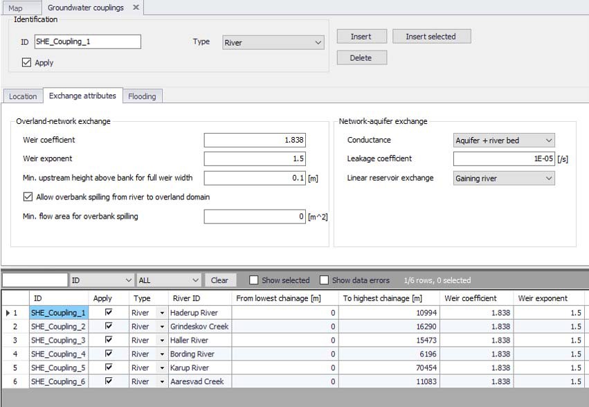
Figure 26.4: MIKE SHE River Links dialogue in the tabular view of the MIKE+ Network Editor

Include all branches button

If the Include all branches button is pressed all the branches in the MIKE+ setup will be copied to the MIKE SHE Links table.

Branches that should not be in the coupling can subsequently be deleted manually and the specifications for the remaining branches completed. Thus, you may have a large and complex hydraulic model, but only couple certain reaches to MIKE SHE. All branches will still be in the hydraulic MIKE 1D model but MIKE SHE will only exchange water with branch reaches that are listed in the MIKE SHE links table.

Note

The Include all branches button will erase all existing links that have been specified.

Location

The branch name, upstream chainage and downstream chainage define the stretch of river that can exchange water with MIKE SHE. A MIKE 1D branch can be sub-divided into several coupling reaches, to allow, for example, different riverbed leakage coefficients for different parts of the river.

7.2 River Aquifer Exchange

Conductance

The river bed conductance can be calculated in three ways.

Aquifer only - When the river is in full contact with the aquifer material, it is assumed that there is no low permeable lining of the river bed. The only head loss between the river and the grid node is that created by the flow from the grid node to the river itself. This is typical of gaining streams, or streams that are fast moving. More detailed information on this option can be found in Aquifer Only Conductance.

River bed only - If there is a low conductivity river bed lining, then there will be a head loss across the lining. In this case, the conductance is a function of both the aquifer conductivity and the conductivity of the river bed. However, when the head loss across the river bed is much greater than the head loss in the aquifer material, then the head loss in the aquifer can be ignored (e.g. if the bed material is thick and very fine and the aquifer material is coarse). This is the assumption used in many groundwater models, such as MODFLOW. More detailed information on this option can be found in River bed only conductance.

Aquifer + Bed - If there is a low conductivity river bed lining, then there will be a head loss across the lining. In this case, the conductance is a function of both the aquifer conductivity and the total conductivity of the between the river and the adjacent groundwater can be calculated as a serial connection of the individual conductances. This is commonly the case, when the aquifer material presents a significant head loss. For example, when the aquifer is relatively fine and the groundwater cells are quite large.More detailed information on this option can be found in Both aquifer and river bed conductance.

Leakage Coefficient - [1/sec]

This is the leakage coefficient for the riverbed lining in units of [1/seconds]. The leakage coefficient is active only if the conductance calculation method includes the river bed leakage coefficient.

Linear Reservoir Exchange

If you are using the Linear Reservoir method for groundwater in MIKE SHE, then by default the Interflow and Baseflow reservoirs discharge uniformly to all the river links within the reservoir. This is generally true in the lower reaches. However, in the upper reaches many rivers discharge to the groundwater system.

In this dialogue, you can define whether or not a branch is a Gaining branch (default) or a Losing branch. If the branch is a:

• Gaining branch, then the leakage coefficient and wetted area are ignored and the rate is discharge from the Baseflow reservoir to the river is calculated based on the Linear Reservoir method.

• Losing branch, then the rate of discharge from the river to the Baseflow reservoir is calculated using:

  Q = water depth * bank width * branch length * leakage coefficient.

The gaining and losing calculations are done in MIKE SHE for every river link within the Baseflow reservoir. For the losing river links, the water level is interpolated from the nearest h-points, the bottom elevation and bank width is interpolated from the nearest cross-sections. The length is simply the cell size. MIKE SHE keeps track of the inflow volumes to ensure that sufficient water is available in the river link.

7.3 Weir Data for overland-river exchange

The choice of using the weir formula for overland-river exchange is a global choice made in the MIKE SHE OL Computational Control Parameters dialogue. If the weir option is chosen in MIKE SHE, then all MIKE 1D coupling reaches will use the weir formula for moving water across the river bank.The weir option is typically used when you want to simulate overbank spilling and detailed 2D surface flow in the flood plains. The following parameters and options are available when you specify the weir option in MIKE SHE. If you chose the Manning equation option in MIKE SHE, then these parameters are ignored.

Weir coefficient and Head exponent

The Weir coefficient and head exponent refer to the C and k terms respectively in Equation 26.9. The default values are generally reasonable. Both the weir coefficient and the head exponent are dimensionless.

Minimum upstream height above bank for full weir width

In Equation 26.9, when the upstream water depth above the weir approaches zero, the flow over the weir becomes undefined. To prevent numerical problems, the flow is reduced linearly to zero when the water depth is below the minimum upstream height threshold. The EUM data type is Water Depth.

Allow overbank spilling

This checkbox lets you define which branches are allowed to flood over their banks. Thus, you can allow flooding from the river only in branches with defined flood plains, or only in areas of particular interest.

If overbank spilling is not allowed for a particular branch, then the overland-river exchange is still calculated using the weir formula, but the exchange is only one way - that is from overland flow to the river.

Minimum flow area for overbank spilling

The minimum flow area threshold prevents overbank spilling when the river is nearly dry. The flow area is calculated by dividing the volume of water in the coupling reach by the length of the reach. So, you can think of this threshold as a minimum (river volume)/(length of river) before overbank spilling can occur. The EUM data type is Flow Area, which by default is m2.

The default value is 1 m3/m length of river. This is quite a small amount of water for most reasonable rivers and should be adjusted based on the river width. For example for the default value of 1 m3/m,

• if the width of your river is 10m wide, then spilling will occur when the water level is 10cm above the bank elevation.
• if the width of your river is 200m wide, then spilling would start when the water level is only 5mm above the bank elevation.

The cell size also plays a role in determining a reasonable threshold value. When a cell is flooded, the entire cell is covered by water. If the cell size is 1000m x 1000m, then a discharge onto the flood plain of 1 m3/m of river will be only 1mm deep across the cell.

Thus, a value of 1-5 m3/m is probably reasonable for small rivers (10-20m wide) and small grid cells(50-100m). For larger rivers (+50m wide) and larger grid cells (200-500m), a value of 10-50 m3/m is probably more reasonable.

7.4 Inundation options by Flood Code

The Inundation method allows specified model grid cells to be flooded if the river water level goes above the topography of the cell. In this case, water from the river is “deposited” onto the flooded cell. The flood water can then infiltrate, or evaporate. However, overland flow between flooded cells and to the river is not calculated. Also, the flooded water remains as part of the river model water balance and is only transferred to MIKE SHE when it infiltrates.

Inundation areas and their associated Flood codes are specified on a coupling reach basis.

Flood Area Option

The following three options are available for the Flood Area Option:

• No Flooding (default) With the No flooding option, the river is confined between the left and right banks. If the water level goes above the bank elevation, then the river is assumed to have vertical banks above the defined left and right bank locations. No flooding via flood codes will be calculated.
• Manual If the Manual option is selected, then you must supply a flood code map in MIKE SHE. This flood code map is used to established the relationship between river h-points and individual model grids in MIKE SHE. MIKE SHE then calculates a simple flood-mapping during the preprocessing that is used during the simulation to assign river water stages to the MIKE SHE cells if the river level is above the topography.
• Automatic The automatic flood mapping option is useful if the river network geometry is not very complex or for setting up the initial flood mapping, for later refinement. The automatic method, maps out a polygon for each coupling reach based on the left and right bank locations of all the cross-sections along the coupling reach. All cells within this polygon are assigned an integer flood code, unique to the coupling reach. The automatic method works reasonably well along individual branches with cross-sections that represent the flood plain. At branch intersections the assigned flood code may not be correct. However, this is often not serious because at river confluences the water levels in the different branches are roughly the same anyway. In any case, the flood code map is available in MIKE SHE’s preprocessed tab, where you can check its reasonableness. Right clicking on the map will give you the option of saving the map to a dfs2 file, which you can then correct and use with the Manual option.

Note

If neither inundation nor overbank spilling is allowed, then the overland flow exchange to the river is one way only. The only mechanism for river water to flow back into MIKE SHE is through baseflow infiltration to the groundwater. If overland flow does spill into the river, there is first a check to make sure that the water level in the river is not higher than the ponded water.

Flood Code

If the Manual option is selected, then you must specify a Flood code for the coupling reach. The flood code is used for mapping MIKE SHE grids to river h-points. You must click on the Flood Code checkbox in Figure 26.4, and then specify an integer flood code file in MIKE SHE. The specified flood code for the coupling reach must exist in the dfs2 Flood Code file. It is important to use unique flood codes to ensure correct flood-mapping.

Bed Topography

Since the flood mapping procedure will only flood a cell when the river water level is above the cell’s topography, accurate flood inundation mapping requires accurate elevation data. If one of the flood options are selected, then you have the option to refine the topography of the flood plain cells based on the actual cross-section elevations or on a more detailed local-scale DEM, if it exists.

• Use Grid Data (default) If Grid Data option is selected, the MIKE SHE topography value is used to determine whether or not the cell is flooded. However, the program first checks to see if a Bathymetry file has been specified.

If a Bathymetry file is available, the topography values of the cells with flood codes are re-interpolated based on the bathymetry data. The bathymetry option is useful when a more detailed DEM exists for the flood plain area compared to the regional terrain model.

• Use Cross-section If the Cross-section option is specified the topography values of the cells with flood codes are re-interpolated based on the cross-section data.

When the cross-section option is selected, the pre-processor maps out a flood-plain polygon for the coupling reach, based on the left and right bank locations of all the cross-sections along the coupling reach. Interpolated cross-sections are created between the available actual cross-sections, if the cross-section spacing is greater than ½ \(\Delta x\) (grid size). All the cross-sections (real and interpolated) are sampled to obtain a set of point values for elevation in the flood plain. The topography values of all cells with the current flood code that are within the flood-plain polygon are reinterpolated using the bilinear interpolation method to obtain a new topography value.

In principle, the Cross-section option ensures a good consistency between MIKE SHE grid elevations and river model cross-sections. There will, however, often be interpolation problems related to river meandering, tributary connections, etc., where wide cross-sections of separate coupling reaches overlap. Thus, you can make the initial MIKE SHE set-up using the Cross-section option and then subsequently retrieve and check the resulting ground surface topography, from the pre-processed data. If needed, the pre-processed topography can be saved to a .dfs2 file (right click on the map), modified and then used as input for a new set-up, now using the Use Grid Data option.

Bed Leakage

If one of the flood options are selected, then you must also specify if and how the leakage coefficient will be applied on the flooded cells. The infiltration/seepage of MIKE SHE flood grids is calculated as ordinary overland exchange with the saturated or unsaturated zone. That is, the leakage coefficient, if it exists, is applied to both saturated exchange to and from the flooded cell and unsaturated leakage from the flooded cell. In the case of the unsaturated leakage, the actual leakage is controlled by either the leakage coefficient or the unsaturated zone hydraulic conductivity relationship - which yields the lowest infiltration rate.

• Use grid data In this case, the leakage coefficient specified in Surface-Subsurface Leakage Coefficient is used. If this item has not been specified, then the leakage coefficient will be calculated based on the aquifer material only.
• Use river data (default) In this case, the Leakage Coefficient - [1/sec] for the coupling reach is actually copied to the flooded cell and used for all flood grid points of the coupling reach. This makes sense if the flood plain is frequently flooded and covered with the same sediments as the river bed. However, in many cases the flood plain material is not the same as the river bed and the infiltration rate can be substantially different.

8. Common MIKE 1D River Error Messages

There are a number of common error messages that you are likely to encounter when using a river model with MIKE SHE.

8.1 Error No 25: At the h-point the water depth greater than 4 times max. depth

This error message essentially says that your river model is unstable. It frequently occurs when there is an inconsistency in your bed elevations at the branch junctions. For example, if the bed elevation of the main branch is much greater than the side branch, then the water piles up and causes this error.

8.2 Warning No 47: At the h-point the water level as fallen below the bottom of the slot x times

This warning message essentially says that your river model is unstable. The slot is a numerical trick that keeps a very small amount of water in the river cross-section when the river is dry. So, when the water level falls below the slot, it implies that your river has dried out. This warning frequently occurs when there is either an inconsistency in your bed elevations or there is an error in your boundary conditions that is keeping water from entering the system.

8.3 Warning No : Bed levels not the same

This warning message is issued when the bed elevation of a side branch is not the same as the main branch. If the difference is small (say a few cm) it can usually be ignored. However, if the side branch is much lower than the main branch then this warning will often be accompanied by Error No 25: Atthe h-point the water depth greater than 4 times max. depth, as the water will pile up and not be able to flow into the main branch. If the side branch is only slightly lower than the main branch or even if they are the same, then backward flows can occur in the side branch when the water level in the main branch rises. If this is realistic fine, but often it is not. More typically, the side branch