Working with Overland Flow and Ponding- User Guide

When the net rainfall rate exceeds the infiltration capacity of the soil, water is ponded on the ground surface. This water is available as surface runoff, to be routed downhill towards the river system. The rate of overland flow is controlled by the surface roughness and the gradient between cells. The direction of flow is controlled by the gradient of the land surface - as defined by the topography. The quantity of water available for overland flow is the available ponded depth minus the detention storage, as well as the losses due to evaporation and infiltration along the flow path.

Overland flow can be a very time consuming part of the simulation. There are many ways to reduce this burden - often without significantly impacting the accuracy of the results.

This Chapter provides additional information and tips to help you understand how overland flow and ponding work, as well as help you speed up your simulations. It is divided into five sections:

• Overland Flow Control - this section describes additional information on parameter values;
• Overland Flow Performance - this section provides additional information on optimizing your overland simulation;
• Multi-cell Overland Flow - this section describe how to include a sub-grid scale topography in your overland flow calculations;
• Overland Drainage - this section describes how to use route ponded water directly to rivers, boundaries and internal depressions; and
• Reduced OL leakage to UZ and to/from SZ - this section describes how to limit exchange across the land surface in areas that are compacted or paved.

1. Overland Flow Control

The overland flow calculations are controlled by parameters and some basic options.

1.1 Principal parameters

The main overland flow parameters are the surface roughness which controls the rate of flow, the depth of detention storage which controls the amount of water available for flow, plus the intial and boundary conditions.

Surface Roughness

The Stickler roughness coefficient is equivalent to the Manning M. The Manning M is the inverse of the commonly used Manning’s n. The value of n is typically in the range of 0.01 (smooth channels) to 0.10 (thickly vegetated

channels), which correspond to values of M between 100 and 10, respectively.

If you don’t want to simulate overland flow in an area, a Manning’s M of 0 will disable overland flow. However, this will also prevent overland flow from entering into the cell.

Detention Storage

Detention Storage is used to limit the amount of water that can flow over the ground surface. The depth of ponded water must exceed the detention storage before water will flow as sheet flow to the adjacent cell. For example, if the detention storage is set equal to 2mm, then the depth of water on the surface must exceed 2mm before it will be able to flow as overland flow. This is equivalent to the trapping of surface water in small ponds or depressions within a grid cell.

Water trapped in detention storage continues to be available for infiltration to the unsaturated zone and to evapotranspiration.

Detention storage also affects the exchange with the river. Only ponded water in excess of the detention storage will flow to the river. Also, flooding from the river will only happen when the water level in the river link is above the topography plus detention storage.

The OL Drainage is also linked to the detention storage. Only the available ponded water will be routed to the OL Drainage network - that is the ponded depth above the detention storage. If you want to route all of the ponded water to the OL Drainage network, then you can use the Extra Parameter: OL Drainage Options.

Initial and Boundary Conditions

In most cases it is best to start your simulation with a dry surface and let the depressions fill up during a run in period. However, if you have significant wetlands or lakes this may not be feasible. However, be aware that stagnant ponded water in wetlands may be a significant source of numerical instabilities or long run times.

The outer boundary condition for overland flow is a specified head, based on the initial water depth in the outer cells of the model domain. Normally, the initial depth of water in a model is zero. During the simulation, the water depth on the boundary can increase and the flow will discharge across the boundary. However, if a non-zero initial condition is used on the boundary, then water will flow into the model as long as the internal water level is lower than the boundary water depth. The boundary will act as an infinite source of water.

Time varying OL boundary conditions

If you need to specify time varying overland flow boundary conditions, you can use the Extra Parameter option Time-varying Overland Flow Boundary Conditions.

1.2 Separated Flow areas

The Separated Flow Areas are typically used to prevent overland flow from flowing between cells that are separated by topographic features, such as dikes, that cannot be resolved within a the grid cell.

In many detailed models, surface drainage on flood plains and irrigation areas is highly controlled. The Separated Flow Areas option allows you to define these drainage control land features in the model.

If you define the separated flow areas along the intersection of the inner and outer boundary areas, MIKE SHE will keep all overland flow inside of the model - making the boundary a no-flow boundary for overland flow.

However, separated flow areas are not respected by the other hydrologic processes, such as the SZ drainage function. Thus, lateral flow out of the model may still occur via SZ drainage, SZ boundary conditions, the river, irrigation control areas, etc. even when the separated flow areas are defined. Therefore, if you use separated flow areas, you should carefully evaluate your results, for example, by using the water balance tool, to make sure that the water flow is behaving as you expect.

Also, you should note that Overland flow cannot cross a river link. So, the cell faces with river links always define a separated flow boundary.

1.3 Output: Overland Flow Velocities

MIKE SHE calculates overland flow based on the diffusive wave approximation, which neglects the momentum. Further, the depth and flow rates are averages for a cell, which does not take into account the actual distribution of velocities and water depths in a natural topography. Finally, if the area of interest is next to a river, then the physical exchange with the river depends on the calculation method used. Even in the best case, exchange between the river and the flood plain is conceptual. There is no velocity calculated for the river-OL exchange, nor is there any momentum transfer between the overland flow and the flow in the river. Water is simply taken from the river and put on the flood plain cell, or vice versa. The rate of exchange depends the water level difference and the weir coefficients used.

Thus, the calculated velocity is less useful for things like damage assessment. If velocities are important, then the MIKE+ 2D Overland module is a much better tool. MIKE SHE, on the other hand, is good at calculating overland water depths, general flow directions and the exchange of ponded water with the subsurface and rivers.

MIKE SHE does, however, generate several output items related to velocity.

Overland flow in the x- and y-direction

The overland flow in the x- and y- in the list of available output items is used for the water balance calculations.

The cell velocity cannot be directly calculated from these because the overland water depth is an instantaneous value output at the end of storing time step. Whereas, the overland flow in the x- and y- directions are mean-step accumulated over the storing time step. Thus, it is the accumulated flow across the cell face on the positive side of the cell.

You may be tempted to calculate a flow velocity from these values. But, you can easily have the situation where the accumulated flow across the boundary is non-zero, but at the end of the storing time step, the water depth is zero. Or, you could have a positive inflow and a zero outflow, which may be misleading when looking at a map of flow velocities.

For example, if your storing time step is a month, your flows will be a monthly average. The flow will be saved at midnight on the last day of the month.

Depending on the timing of your events, you could easily have a high average flow and a zero depth.

H Water Depth, P flux and Q flux

The P and Q fluxes are instantaneous fluxes across the positive cell faces of the cells. These are found in a separate _flood.dfs2 results file, along with the H Water Depth. This file is the same format as the MIKE 21 output files generated by the MIKE+ 2D Overland module. Thus, you can use this file to generate flood maps etc in, for example, the Flood Modelling Toolbox, or the Plot Composer.

You can also add these values to create flow vectors in the Results Viewer.

TS average, TS min, and TS max

Three calculated depths and velocities are available. These are the Average, Minimum and Maximum velocities and depths over the storing timestep.

These values could be useful, for example, when evaluating susceptibility to erosion, or to calculate a flood hazard indicator.

2. Overland Flow Performance

The overland flow can be a significant source of numerical instabilities in MIKE SHE. Depending on the setup, the overland flow time step can become very short - leading to very long.

Overland flow has both an Implicit and Explicit solver. Your choice of solver affects both the accuracy of your results and the simulation run time.

The Implicit solver is faster than the Explicit solver because it can run with longer time steps. However, the it must iterate to converge on a solution. Thus, if each time step takes several iterations because of the dynamics of the overland flow, then the implicit solver can become slow. The most obvious sign of poor convergence is the presence of warning messages in the project- name_WM_Print.log file about the overland flow solver not converging. You may be able to live with a few warning messages, but the if the Implicit solver frequently fails to converge then this will significantly slow down your simulation. If this happens, then you have a few options.

The first option is to reduce your OL time step. This make increase the stability of the solver and actually reduce your run times. You can also increase the convergence criteria. This will decrease the accuracy, but if there is a troublesome area outside of your area of interest, then this may be acceptable.

If you switch to the Explicit solver, then the time step becomes dynamic depending on the Courant criteria. This will likely reduce your numerical instabilities because the Courant criteria is very restrictive, but the simulation is likely to be slower. However, the difference may not be that great if you are having a lot of convergence problems.

2.1 Stagnant or slow moving flow

The solution of overland flow is sensitive to the surface water gradient. If the surface water gradient is very small (or zero), then a numerically stable solution will generally require a very short time step.

Slow moving flow is a problem when you have long term ponded water, for example in wetlands. If you are only interested in the water levels in the wetland areas, but not the flow velocity and flow directions, then solving the overland flow equations is not necessary for decision making.

If you want to turn off the overland flow solver in slow moving or stagnant areas, then you can convert these areas to flood codes and allow the river model to control the water levels. Lateral overland runoff to these areas will still be calculated, as will evapotranspiration and infiltration. For more detail on using Flood Codes, see Overland Flow Exchange with Rivers.

An alternative is to turn off the overland flow calculation in these cells. You can turn off the overland flow in a cell by setting the Manning’s M number to zero. However, this also turns off the lateral overland inflow into the cell, as well.

Another option is to use the detention storage parameter to restrict the amount of available water. In this case, overland flow is allowed into and out of the cell, but overland flow is not actually calculated until the depth of water in the cell exceeds the detention storage.

The Threshold gradient for overland flow (see next Section) is also a way to reduce the influence of stagnant water on the time step. However, you cannot specify a spatially varying threshold. So, the appropriate value may be difficult to select if you want to restrict flow in one area, yet keep surface flow in other less stagnant areas.

If you are using the Explicit OL solver, there are several dfs2 output options that make it easier to find the model areas that are contributing to reducing the time step. These include:

• Mean OL Wave Courant number,
• Max OL Wave Courant number, and
• Max Outflow OL-OL per Cell Volume.

2.2 Threshold gradient for overland flow

In flat areas with ponded water, the head gradient between grid cells will be zero or nearly zero. As the head gradient goes to zero, \(\Delta t\) must also become very small to maintain accuracy. To allow the simulation to run with longer time steps and dampen any numerical instabilities in areas with low lateral gradients, the calculated intercell flows are multiplied by a damping factor when the gradients are close to zero.

Essentially, the damping factor reduces the flow between cells. You can think of the damping function as an increased resistance to flow as the gradient goes to zero. In other words, the flow goes to zero faster than the time steps goes to zero. This makes the solution more stable and allows for larger time steps. However, the resulting gradients will be artificially high in the affected cells and the solution will begin to diverge from the Manning solution. At very low gradients this is normally insignificant, but as the gradient increases the differences may become noticeable. Therefore, the damping function is only applied when the gradient between cells is below a user-defined threshold.

The details of the available functions can be found in the Section Low gradient damping function.

For both functions and both the explicit and implicit solution methods, each calculated intercell flow in the current time step is multiplied by the local damping factor, FD, to obtain the actual intercell flow. In the explicit method, the flow used to calculate the Courant criteria are also corrected by FD.

The damping function is controlled by the user-specified threshold gradient (see Common stability parameters for the Overland Flow), below which the damping function becomes active.

The choice of appropriate threshold value depends on the slope of the flow surface. Based on both actual model tests in Florida and synthetic setups, the following conclusions can be reached:

• A Threshold gradient greater than the surface slope can lead to excessive OL storage on the surface that takes a long time to drain away.
• A Threshold gradient equal to the surface slope is often reasonable, but there may still be some excess storage on the surface.
• Threshold values less than the surface slope typically cause rapid drainage and give nearly the same answers.
• Threshold values below 1e-7 do not significantly improve the results even if the topography is perfectly flat.
• In general, you should used the highest value possible. Lower values may increase accuracy but at the expense of run time.

Therefore, we can safely recommend a Threshold gradient in the range of 1e- 4 to 1e-5, with a default value of 1e-4. For many floodplains, 1e-4 or 1e-5 should be sufficient. In flood plains with very flat relief, 1e-6 may be used. Lower values are probably never necessary.

Since most discharge happens during and immediately after an event, the threshold gradient is likely to be most important when there is significant ponding that lasts over several time steps and drains to a boundary or the river. Ponded water that infiltrates or evaporates and experiences limited lateral flow will not be affected by the Threshold value.

If the topography slope requires a low Threshold, but the solution is unstable at low threshold values, solution stability may be improved with the Explicit solver by reducing the Maximum Courant number until the solution becomes stable. With the Implicit solver, you may need to change the solver parameters.

Performance Impact

A low Threshold gradient will increase your simulation time. So, the final value that you use, may be a compromise between simulation length and accuracy of the flow in low gradient conditions.

If you have stagnant ponded water in your model, then the intercell gradient in these areas will be nearly zero. If you lower your Threshold gradient, your simulation performance may be adversely impacted, simply because the OL solver will begin to calculate flow sloshing back and forth in these areas. Not only will the OL solver have to work harder, the OL time step will likely also decrease because of the very low gradients. Thus, the Threshold gradient effectively reduces intercell flow in stagnant areas to zero allowing the Courant criteria to be satisfied at much higher time step lengths.

3. Multi-cell Overland Flow

The main idea behind the 2D, multi-grid solver is to make the choice of calculation grid independent of the topographical data resolution. The approach uses two grids:

• One describing the rectangular calculation grid, and
• The other representing the fine bathymetry.

The standard methods used for 2D grid based solvers do not make a distinction between the two. Thus, only one grid is applied and this is typically chosen based on a manageable calculation grid. The available topography is interpolated to the calculation grid, which typically does not do justice to the resolution of the available data. The 2D multi-grid solver in MIKE SHE can, in effect, use the two grids more or less independently.

In the Multi-cell overland flow method, high resolution topography data is used to modify the flow area used in the St Venant equation and the courant criteria. The method utilizes two grids a fine-scale topography grid and a coarser scale overland flow calculation grid. However, both grids are calculated from the same reference data - that is the detailed topography digital elevation model.

In the Multi-cell method, the principle assumption is that the volume of water in the fine grid and the coarse grid is the same. Thus, given a volume of water, a depth and flooded area can be calculated for both the fine grid and the coarse grid. See Figure 30.1.

In the case of detention storage, the volume of detention storage is calculated based on the user specified depth and OL cell area.

During the simulation, the cross-sectional area available for flow between the grid cells is an average of the available flow area in each direction across the cell. This adjusted cross-sectional area is factored into the diffusive wave approximation used in the 2D OL solver. For numerical details see Multi-cell Overland Flow Method in the Reference manual.

The multi-grid overland flow solver is typically used where an accurate bathymetric description is more important than the detailed flow patterns. This is typically the case for most inland flood studies. In other words, the distribution of flooding and the area of flooding in an area is more important than the rate and direction of ingress.

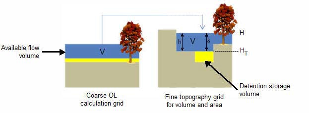
Figure 30.1: The constant volume from the coarse grid is transferred to the fine scale grid

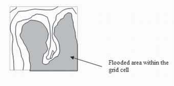
Figure 30.2: Flooded area is a function of the surface water level in the grid cell.

Elevations

The elevation of the coarse grid nodes and the fine grid nodes are calculated based on the input data and the selected interpolation method. However, the coarse grid elevation is adjusted such that it equals the average of the fine grid nodal elevations. This provides consistency between the coarse grid and fine grid elevations and storage volumes. Therefore, there may be slight differences between the cell topography elevations if the multi-cell method is turned on or off. This could affect your model inputs and results that depend on the topography. For example, if you initial water table is defined as a depth to the water table from the topography.

3.1 Evaporation

Evaporation is adjusted for the area of ponded water in the coarse grid cell. That is, evaporation from ponded water is reduced by a ponded area fraction, calculated by dividing the area of ponding in the fine grid cell by the total cell area.

The ET from soil evaporation is also reduced to the areas where there is not ponding.

Total transpiration does not need to be adjusted for the non-ponded area because evaporation from the ponded area is calculated prior to transpiration, and this is already adjusted for the ponded area in the cell. Thus, if the cell is fully ponded, then the Reference ET will be satisfied from ponded storage and there will be no transpiration. If the cell is only partially ponded, then the area fraction of the RefET will be first extracted from the ponded water and the remainder from the root zone. Since, there is only one UZ column to extract from, the entire root zone will be available for transpiration.

The Extra Parameter option,Transpiration during ponding, allows transpiration from the root zone beneath ponded areas. In this case, transpiration is calculated before evaporation from ponding. This option includes a reduction factor to account for the reduced ET under saturated conditions. The application of this factor will be changed so that it only applies to the ponded fraction of the cell.

3.2 Infiltration to SZ and UZ with the Multi-Grid OL

If ponded water is flowing between cells, the multi-scale topography will ensure that only the lowest part of each cell will be flooded, and the rate of flow between the cells will be adjusted for the flooded depth. However, the infiltration also needs to be adjusted to account for the fact that there is a driving pressure head in some parts of the cell.

Infiltration to UZ

The UZ infiltration is calculated based on three UZ calculations: one for the ponded fraction of the cell, one for the non-ponded fraction of the cell and finally a calculation is made using the area weighted infiltration of the two first UZ calculations. The last step is needed as there is only one UZ column below the multi-cells.

In a MIKE SHE simulation without multi-cell infiltration, the engine calculates an average storage depth, which is available for infiltration. This storage depth is then used for the infiltration calculations. The storage depth is calculated as follows:

1. Assuming that the OL depth from the previous OL time step is known,
2. the OL depth is updated using the current net precipitation and any sink and source terms (irrigation, by pass flow, paved area drainage etc.). Noting that:
   • Bypass flow is extracted from the net precipitation before the infiltration calculation, and
   • OL Drainage is also extracted before the infiltration calculation. The updated OL depth is used for the infiltration calculation;
   • If the reduced contact option is used, the leakage coefficient is used to calculate the maximum infiltration rate.

When using the multi-cell infiltration, the infiltration is calculated based on three cases which depend on the ponded area fraction from the latest OL time step:

1. Non ponded (Ponded Area Fraction = 0). Only one infiltration calculation based on the available storage depth. This is done in the same way as a situation without the multi-cell option.
2. Fully ponded (Ponded Area Fraction = 1). Only one infiltration calculation based on the available storage depth. This is done in the same way as a situation without the multi-cell option.
3. Partly ponded (0 \< Ponded Area Fraction \< 1). Three infiltration calculations are made; ponded area, non-ponded area and a final calculation using the area weighted storage depth.

In the partly ponded case, it is assumed that the net-precipitation is equally distributed across the whole cell, while ponding from the previous OL time step only occurs in the ponded part of the cell. For the infiltration calculation in the non-ponded are, the available water depth is calculated as

Equation 30.01

The remaining part of the available water (ponding + precipitation on the ponded part) is scaled to an equivalent water depth in the ponded area:

Equation 30.02

where OLDepth is the depth of ponded water from the previous time step, and PAreaFrac is the ponded area from the previous time step.

Disabling multi-cell infiltration

Multi-cell infiltration is automatically activated when the multi-cell option is invoked. However, an Extra Parameter option is available if you want to disable this function - perhaps for backwards compatibility with older models.

Parameter Name	Type	Value
disable multi-cell infiltration	Boolean	On

When this is specified, the infiltration will be calculated based on the values of the course grid, and any ponding occurring in any sub-grid cells will not be included.

3.3 Multi-cell Overland Flow + Saturated Zone drainage

The topography is often used to define the SZ drainage network. Thus, a refined topography more accurately reflects the SZ drainage network.

The SZ drainage function uses a drain level and drain time constant. The drain level defines the depth at which the water starts to drain. Typically, this is set to some value below the topography to represent the depth of surface drainage features below the average topography. This depth should probably be much smaller if the topography is more finely defined in the sub-grid model. The drain time constant reflects the density of the drainage network. If there are a lot of drainage features in a cell then the time constant is higher and vice versa.

Details related to the use of the Multi-cell OL with the SZ Drainage function are found along with the rest of the user guidance on SZ Drainage in the section: Saturated Zone drainage + Multi-cell Overland Flow.

3.4 Test example for impact on simulation time

The increased accuracy of the multi-cell overland flow method does not come for free. There is a performance penalty when you turn on the multi-cell option. However, the penalty relative to the increased accuracy of water depths is small.

A test done on a large, complex model in Florida, USA illustrates the performance penalty of the multi-cell method.

In the model the grid cell size is 457.2 m (1500 ft). However, a high resolution (5-ft) DEM is available for the whole model domain based on LIDAR data.

This makes it attractive to use of higher resolution map with the Multi-cell option to account more accurately for the OL flow between 1500-ft grid cells.

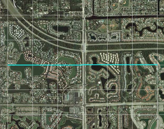
Figure 30.3:Aerial photo of part of the model area

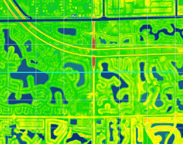
Figure 30.4:5-foot LIDAR data for part of the model area

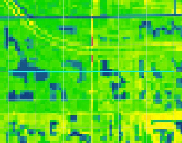
Figure 30.5:Interpolation of the 5-foot LIDAR data to the 125ft model grid

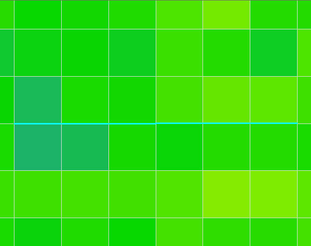
Figure 30.6:Interpolation of the 5-foot LIDAR data to the 1500ft model grid

Impact on simulation time

In this test, we tested multi-cell factors of 1, 2, 3, 4, 6, and 12. The smallest grid size was 125-ft, which is 12 times smaller than the coarse 1500-ft grid.

The following graphs illustrate the impact of the multi-grid option on the running times for the test model. Figure 30.7 shows that the OL run time increases linearly with higher multi-cell factors. In the test model, a multi-cell factor of 12 caused the OL portion of the simulation time took 30 times longer. Figure 30.8 shows that the multi-cell factor also impacts the run time for the river model. However, this impact is not linear, with the impact on MIKE 1D leveling off after a multi-cell factor of four.

The test model run time is dominated by MIKE 1D. In this case, the original run time for the OL is not very long and the multi-cell factor increases the OL run time considerably. However, as a fraction of the total run time, the OL is still small. When the OL cells are subdivided, there is probably some significant changes in the lateral inflow to MIKE 1D. However, as the multi-cell factor increases, the increased resolution of the inflows is not significant above a factor of about four.

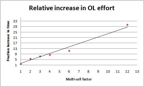
Figure 30.7:Increase in OL run time as a function of multi-cell factor

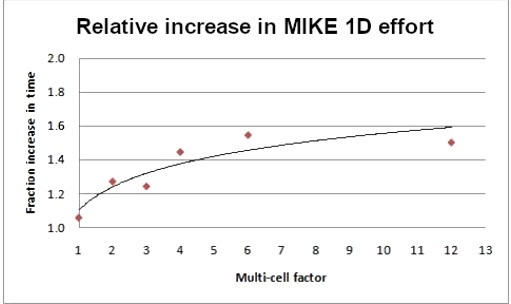
Figure 30.8:Increase in the river model run time as a function of the multi-cell factor.

Impact on model results

The model contains a mix of natural, urban, and agricultural areas. The model also includes a complex river network with the relevant man-made canals and structures, and most of the natural flow ways. However, there is a natural flow way in the southeast part of the model that is not conceptualized in the river model. Since, the surface water flow in this area is relying only on overland flow, the multi-cell option should significant changes in the OL flow prediction in this natural flow way.

In urban and agricultural areas, the drainage and the OL flow components in MIKE SHE route the water into the canal network. The drainage component would keep the water table level below the ground most of the time in those areas. However, it is of interest to test the OL flows predicted with the multicell option in those areas during storms events.

3.5 Limitations of the Multi-cell Overland Flow Method

In principle, all of the exchange terms in MIKE SHE could be adjusted to reflect the fine scale water levels and flooded areas. However, some of these are easier to implement than others and of greater importance. Thus, in current release, the exchange with the river, as well as UZ and SZ, depend only on the coarse scale grid elevations.

Overland flow exchange with rivers

Overland flow exchange with rivers does not consider the multi-cell method. That is, flow into and out of the River Links is controlled by the water level calculated from the elevation defined in the coarse grid cell. Likewise the flow area for exchange with the river is calculated as the coarse water depth times the overall grid size. Also, the elevation used when calculating flood inundation with flood codes only considers the average cell depth of the coarse grid. See Overland Flow Exchange with Rivers.

However, if you choose to modify the topography based on a bathymetry file, or the river cross-sections, then this information will be used when calculating the multi-cell elevations.

3.6 Setting up and evaluating the multi-grid OL

The multi-cell overland flow method is activated in the OL Computational Control Parameters dialogue. In this dialogue, you can check on the option and then specify a sub-division factor. The coarse grid will be divided into this number of cells in both directions. That is, for a factor of two, the coarse grid will be divided into four cells. Likewise a factor of five will lead to 25 fine cells per coarse grid cell.

Pre-processed data

When you enable the Multi-grid OL option the following new items will be available in the preprocessed data:

• Multi-Cell ground levels (subscale topography) In Figure 30.9, two interpolations of the same DEM are shown. The top figure is a plan view of the interpolation to a 100m grid resolution and a 25m grid resolution respectively. The bottom figure is a cross-section across the middle of the top figure, where you can clearly see the more accurate resolution of the drainage features.

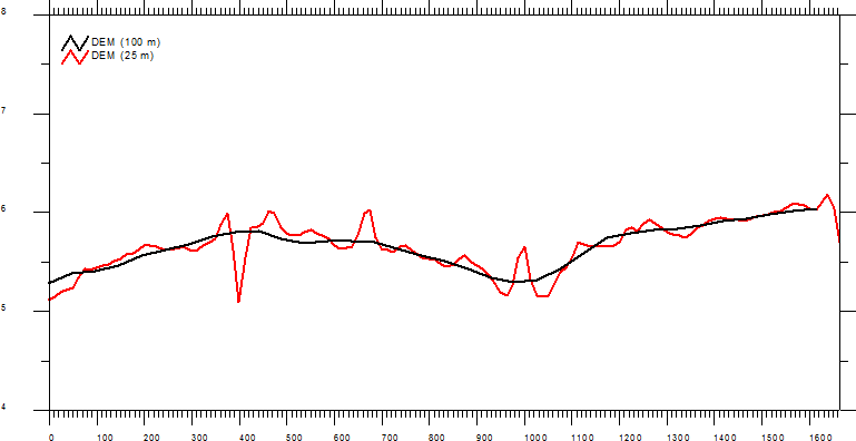
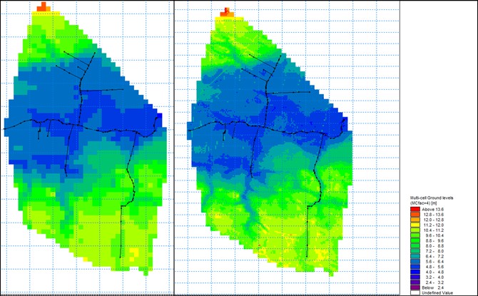
Figure 30.9:Example of preprocessed data - topography using a 100 meter resolution and a sub-scale factor of 4 (25 m sub-scale resolution)

When SZ Drainage is also active, then the following items are also available:

• Max. MC Drain Level - displays the maximum drain level of the sub-cells within each of the model cells
• Min MC Drain level - displays the minimum drain level of the sub-cells within each of the model cells
• Min MC Drain Depth - displays the minimum drain depth of the sub-cells within each of the model cells
• Max MC Drain Depth - displays the maximum drain depth of the sub-cells within each of the model cells

Additional results options

When the Multi-grid OL option is active, the following additional items will be available in the result items:

• Depth of Multi-Cell overland water - displays the depth of overland water using the sub-scale resolution
• Multi-Cell overland water elevation - displays the overland water elevation using the sub-scale resolution

4. Overland Drainage

In natural systems, runoff does not travel far as sheet flow. Rather it drains into natural and man-made drainage features in the landscape, such as creeks and ditches. Then, it generally discharges into streams, rivers or other surface water features. In urban areas, it may discharge into storm water retention basins designed to capture runoff.

The amount of runoff generated by MIKE SHE depends on the density of the stream network defined in the river model. If the stream network is dense, then you will get more runoff in the model because the lateral travel time to the streams will be short, and the infiltration and evaporation losses will be smaller.

Fine-scale, natural and man-made drainage systems are difficult to simulate in MIKE SHE using the traditional finite difference Overland Flow method.

This is largely because the drainage features are often smaller than the grid scale, and shallow overland flow will not travel far laterally before it infiltrates or evaporates.

In large catchments, it may be impractical to define the detailed natural drainage network. In urban catchments, the detail of the drainage network may be either unknown or impractical to define.

The overland drainage (OL drainage) option was introduced to alleviate some of these issues. Conceptually, the OL drainage is the similar to the SZ drainage in that a drainage network is calculated based on a downhill flow path from each node until it reaches a stream, a boundary, or a local depression.

A key difference from the SZ Drainage feature is that the OL Drainage includes an intermediate storage. The SZ Drainage is instantly added to the destination, whereas the OL Drainage is first added to an internal storage. Technically, this internal storage is located “on the cell”, not “in the drain”.

Thus, any cell that is generating OL drainage will also have an amount of OL drain storage. The amount of OL drain storage retained on the cell depends on the outflow time constant. This allows you to simulate a rapid drainage of rainfall, but a slower discharge to the receiving destination. Effectively, this is the same as having storage in a drainage network, but the drainage flows from different cells are not summed together, and there is no physical drainage network to interact with while the water is in storage.

The overland drainage function has been designed to facilitate a flexible definition of storm water drainage in both natural and urbanized catchments. In particular, the overland drainage function supports the following features:

• In urban areas, paving and surface sealing (e.g. roof tops) limits infiltration and enhances runoff.
• Ponded water and rainfall are routed to user-defined locations (boundaries, depressions, manholes and streams).
• The time varying storage in the drainage system is accounted for by different inflow and outflow rates.
• Drainage rates can be controlled by drain levels, drainage time constants and maximum flow rates.
• Drainage is restricted if the destination water level is higher than the source water level.
• Urban development over time can be simulated by time varying drainage parameters.
• Infiltration and overland flow are calculated normally for ponded water that does not drain in the current time step.

Conceptually, the overland drainage function is shown in Figure 30.10.

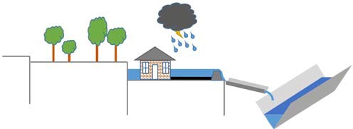
Figure 30.10:Conceptualization of the overland drainage function

Calculation Order and Time Step

The OL drainage is calculated explicitly in a particular order with respect to the other hydrologic processes. However, the exact order depends on what UZ solver is being used. In all cases interception is calculated first. When using the Richards- or the gravity-solver, ET will be calculated before OL drainage, when using the 2-layer UZ solver ET will be calculated after drainage.

After the drainage calculation any remaining precipitation will be added to the remaining ponded water.

If there is any ponded water remaining on the cell after the drainage has been removed, then it will be subject to other processes in the following order:

1. Infiltration to the unsaturated zone;
2. If the groundwater table is at/above ground: direct OL SZ exchange and
3. Finally, Lateral Overland Flow will be calculated to the adjacent cells.

The overland drainage is calculated for every cell independently. That is, the drainage that is calculated is not added to the destination cells until the end of the calculation for all the cells. This prevents circular drainage, and means that the order in which the calculation occurs is not relevant. After the ponded drainage is calculated, the water depths in all the cells are updated - both sources and destinations. The calculation of ET, infiltration and lateral OL flow is based on the updated ponded depths.

Note

When using OL Drainage together with UZ (Richards or gravity) the time spent for the drainage calculation will be accounted for as UZ time. With- out UZ or when using the 2-layer method, the time spend for the drainage calculation adds to OL time.

4.1 Specifying Overland Drainage

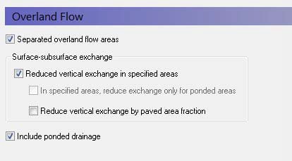
Overland drainage is specified by selecting the Include overland drainage checkbox in the Overland Flow dialog. This will activate the Overland drainage dialog and the default additional data tree items.

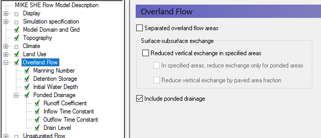
The options for defining OL Drainage are selected in the overland drainage dialog:

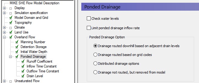
There are two check box options for controlling the OL Drainage:

Check water levels

For a flow from the cell into the drain or if the destination of the OL drainage is a river or an internal depression, the target will have a water level. If you chose the option to check water levels and the target water level is higher than the ground level and higher than the level of detention storage (for flow into the drain) or higher than the drain level (for flow out of the drain) then it will inhibit flow, as it reduces the driving head difference. In other words, this option causes the destination water level to be considered when determining the drain base level zDr0 (see equation 29.24).

The water level inside the drain is calculated based on the OL Drain level plus the volume of water in the OL Drain storage divided by the full cell area.

If the levels are not considered to represent the physical situation, then this option can be turned off. In this case the target water level will be ignored, and any calculated flow will be added to the target. There is no limit on the amount of water that can be stored inside the drain.

Limit inflow rate to OL Drain Storage

The flow rate into the drain is controlled by the drain inflow time constant. Usually, it is large enough to ensure that all available ponding and rainfall will be routed into the drain in the current time step. However, often the conveyance through the drain is restricted by structures such as a culvert. This is addressed by an option for specifying a maximum discharge rate into the drain. The maximum inflow rate can be specified as a constant value or a distributed (dfs2) value.

The maximum inflow rate can be used to control the inflow to the OL drainage system. At every time step, the calculated drainage volume will be checked against the maximum drainage rate. Thus, ponded water will be retained on a grid cell and can be drained later at a controlled rate into the drainage system. While the water is ponded, it will be subject to infiltration, OL flow and

ET. The rate of leakage below the cell can be controlled by the Surface-Subsurface Leakage Coefficient.

The way the overland drainage is calculated, it is the UZ time step average of flow and does not necessarily represent the maximum drain flow. If the correct application of the limited drain inflow rate is important, the length of the UZ time step during a rain event can be controlled using the Precipitation-dependent time step control parameters (see 3.4.3 Controlling the Time).

Note

Prior to Release 2017, this was called the “Max Storage Change Rate” with Item Type [Storage Change Rate] and default EUM Units of [mm/hour]. There is no automatic backwards compatibility conversion for this. If an existing model uses this option, a uniform value has to be manually converted to the new units - Default units [m3/s]. If a dfs2 file is used, the Item Type also needs to be converted to the new Item Type [Discharge].

Destination options for OL Drainage

The default option is to calculate the drainage destination by looking downhill until a river, boundary or local depression is reached. The elevation for calculating this is the Drain Level. Typically, this will be the same as the Topography (default). However, it could be different, for example, in urban areas where the drain level might be based on sewer inverts.

If Drain codes are selected, then the Drain Levels are used only within the cells that have the same Drain code.

4.2 Runoff Coefficient

The OL Drainage is calculated from ponded water and net rainfall. However, the order of operations in the three UZ solvers differs: When using the Richards and Gravity solvers interception and ET are calculated before the OL drainage (i.e. net rainfall = rainfall minus leaf interception minus ET). With the 2Layer Water Balance model interception is calculated first, followed by OL drainage and ET (i.e. net rainfall = rainfall minus leaf interception).

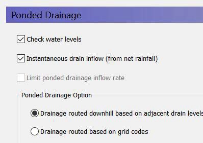
If the option "Instantaneous drain inflow from net rainfall" is not selected, then the drainage runoff coefficient will simply be a scaling factor applied after calculating drain inflow from net rainfall and ponding left over from the previous time step. Conceptually then it can be seen as an area fraction contributing to OL drainage. If at the end of the time step there is still ponded water in the cell, the drainage calculation will be applied to the remainder again in the next time step. Thus, the ponded water will eventually drain away.

However, if the option "Instantaneous drain inflow from net rainfall" is selected, then any ponded water will be neglected, and the specified fraction of net rainfall will be immediately added into the OL drainage storage.

The OL Drainage is also linked to the detention storage. By default, only the available ponded water will be routed to the OL drainage network - that is the ponded depth above the detention storage. If you want to route all ponded water to the OL Drainage network, then you can use an Extra Parameter found in OL Drainage Options.

The OL Drainage function does not check to make sure that you do not create any physically impossible feedback loops. So, flood code cells, and overbank spilling from the river should not be directed to cells where OL Drainage is active. If this happens, you may encounter excessive feedback between MIKE SHE overland flow and the river.

Note

The OL Drainage is calculated on the UZ time step, and stored in the UZ output file. Thus, the OL Drainage depends on the UZ time step length, and the calculated flow will be the UZ time step average. This could affect limiting the drain inflow rate (if specified), because the average value in a long time step could be significantly lower than the actual peak during that time. Also, the division of rainfall and ponding between drainage, infiltration and OL flow may be less accurate using long time steps. The length of the UZ time step during rainfall events can be controlled using the Precipitation- dependent time step control parameters (see 3.4.3 Controlling the Time).

4.3 Time constants

The time constant (or leakage factor) for OL Drainage Inflow controls the rate of water entering the drain storage. The time constant for Outflow controls the rate of water draining to the destination. If the Outflow time constant is sufficiently large, the drain storage will not accumulate any water. In this case, inflow to the drain will be instantly discharged to the destination.

The default value for both time constants is 0.001 1/s. This is quite high and will normally drain nearly all ponded water from the cell. Since the output time constant by default is high, the default storage will be very low. This will normally result in a very sharp peak in your streams in response to the instantaneous drainage of rainfall to the streams.

During model calibration, you can start decreasing the outflow time constant to dampen these drainage peaks.

4.4 OL Drainage Reference System

The OL Drainage function requires a reference system for linking the drainage to a recipient node or cell. The recipient can be a river node, another OL grid cell, or a model boundary.

There are four different options for setting up the drainage source-recipient reference system.

Drainage routed downhill based on adjacent drain levels

The reference system is created automatically by the pre-processor using the slope of the drains calculated from the drainage levels in each cell.

Thus, the pre-processor calculates the drainage source-recipient reference system by

1. looking at each cell in turn and then
2. looking for the neighbouring cell with the lowest drain level.
3. If this cell is an outer boundary cell or contains a river link, the search stops.
4. If this cell does not contain a boundary or river link, then the search is repeated with the next downstream neighbour until either a local minimum is found or a boundary cell or river link is found.

The result of the above search from each cell is used to build the source- recipient reference system.

If local depressions in the drainage levels exist, the OL nodes in these depressions may become the recipients for a number of drain flow producing nodes. This often results in the creation of a small lake at such local depressions.

The drain-slope based reference system has been used in MIKE SHE for many years in SZ and works well in most situations. However, when MIKE SHE is applied where there is very little surface relief, it is often difficult to establish a suitable reference system based on the surface topography/drain slopes. In flat areas, this may generate many undesired local depressions, which may receive drainage water from a large area, thus generating lakes in places where there should not be a lake.

If the drain level is perfectly flat, drainage is turned off. In other words, if the drain-slope method cannot find a downhill neighbour because all the neighbours have the same elevation as the cell, the drain slope method assumes that the cell is a local depression. However, the depression has no

sources of drainage except itself. Thus, the drainage function is effectively turned off.

Tip

MIKE SHE considers a grid point to be a local depression even if the drainage level in the four surrounding model grids is only 1 mm higher. The only way to avoid such problems is to create a drain level map that does not contain artificial local depressions. For large models this may be difficult and time consuming. In this case, one of the other drainage options may be better. The command line tool MSheFillDepressions.exe in your MIKE installation directory can be used to fill depressions. To get help for that tool call it with the argument '--help'.

Remember, the drainage is routed to a destination. It does not physically flow downhill. The drain levels are only used to build the drainage source-recipient reference system, and to calculate the amount of drainage.

Drainage routing based on grid codes

This method is often used when the topography is very flat, which can result in artificial depressions, or when the drainage system is very well defined, such as in urban applications.

In this method, the drainage levels and the time constants are defined as in the previous method and the amount of drainage is calculated based on the drain levels and the time constant.

If the drainage routing is specified by Drain Codes, a grid code map is required that is used to restrict the search area for the source-recipient reference system. In this case, the pre-processer calculates the reference system within each grid code zone, such that all drainage generated within one zone is routed to recipient nodes with the same drain code value.

When building the reference system, the pre-processor looks at each cell and then

1. looks for the nearest cell with a river link with the same grid code value,
2. if there is no cell with a river link, then it looks for the nearest outer boundary cell with the same grid code,
3. if there are no cells with outer boundary conditions, then it looks for the cell with the same grid code value that has the lowest drain level. In this case, the reference system is calculated as if it was based on Drain Levels (see previous section).

The result of the above search for each cell is used to build the source-recipient reference system.

The above search algorithm is valid for all positive Drain Code values. However, all cells where

• Drain Code = 0 - will not produce any drain flow and will not receive any drain flow, and
• Drain Code \< 0 (negative) - will not drain to river links, but will start at Step 2 above and only drain to either an outer boundary or the lowest drain level.

Tip: One method that can be used is to specify one Drain Code value for the entire model area (e.g. Drain Code = 1). Thus, all nodes can drain and any drain flow is routed to the nearest river link. If there are no rivers, the drain flow will be routed to the nearest boundary. If you want to route all drain flow to the boundaries instead of the rivers, a negative drain code can be specified for the entire area (e.g. Drain Code = -1).

Distributed drainage options

Choosing this method, adds the Option Distribution item to the data tree. With the Option Distribution, you can specify an integer grid code distribution that can be used to specify different drainage options in different areas of your model.

• Code = 1 - In grid cells with a value of 1, the drainage reference system is calculated based on the Drain Levels.
• Code =2 - In grid cells with a value of 2, the drainage reference system is calculated based the Drain Codes.
• Code = 3 - Drainage in grid cells with a value of 3 is routed to a specified river branch and chainage. At the moment, this options requires the use of Extra Parameters and is described in OL Drainage to Specfied River H-points.
• Code = 4 - Drainage in grid cells with a value of 4 is routed to a specified sewer manhole. This option is described in the section in Working with Sewers - User Guide.

Drain flow not routed, by removed from model

The fourth option simply removes the water from the model. This is equivalent to routing all the drainage to a boundary.

Drain Code Example

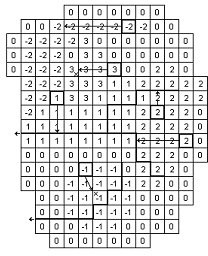
• The grid cells with Drain Code 3 drain to a local depression since no boundary or river link is found adjacent to a grid with the same drain code.
• The grid cells with Drain Code 1 or 2 drain to nearest river link located adjacent to a grid with the same drain code.
• The grid cells with drain code 0 do not contain drains and thus no drainage is produced.
• The grid cells with Drain Code -1 drains to local depression since no boundary is found adjacent to a grid with the same drain code.
• The grid cells with Drain Code -2 drains to nearest boundary grid with the same drain code.

4.5 Preprocessed data

During the preprocessing, each active drain cell is mapped to a recipient cell. Then, whenever drainage is generated in a cell, the drain water will always be moved to the same recipient cell. The drainage source-recipient reference

system is displayed in the following two grids in the Pre-processed tab, under the Overland Flow:

• Drain Codes - The value in the pre-processed Drain Codes map reflects the Option Distribution specified. For example, those cells with an Option Distribution equal to 1 (Drainage routed based on Drain Levels) will have a pre-processed Drain Code equal to 0, because the Drain Codes are not being used for those cells.
• Drainage to local depressions and boundary - This grid displays all the cells that drain to local depressions or to the outer boundaries. All drainage from cells with the same negative value are drained to the cell with the corresponding positive code. If there is no corresponding positive code, then that cell drains to the outer boundary, and the water is simply removed from the model. Cells with a delete value either do not generate drainage, or they drain to a river link.
• Drainage to river - This grid displays the river link number that the cell drains to. Adjacent to the river links, the cells are labeled with negative numbers to facilitate the interpretation of flow from cells to river links. Thus, in principle, all drainage from cells with the same positive code are drained to the cell with the corresponding negative code.

However, this is slightly too simple because the cells actually drain directly to the river links. In complex river systems, when the river branches are close together, you can easily have cells connected to multiple branches on different sides. In this case, the river link numbers along the river may not reflect the drainage-river link reference used in the model.

If you want to see the actual river links used in all cells, you can use the Extra Parameter, OL Drainage to Specified River H-points, to generate a table of all the river link-cell references in the PP_Print.log file.

4.6 Time varying OL Drainage parameters

In projects where you want to simulate the build out of an OL Drainage network over time, or changes in the OL Drainage time constants over time, then you can use time varying parameters. Without this you would have to hot start your simulation at regular time intervals with the new OL Drainage parameters.

Note

If you specify time varying OL Drainage parameters, you will not be able to use any of the drainage routing methods that depend on the OL drain level. The drain level methods are not allowed because the source-recipient reference system is only calculated once at the beginning of the simulation.

The preprocessor checks this and gives an error if you have specified

• option 1 (routing based on levels), or
• option 3 (distributed options) AND any of the distributed option codes are 1 (routing based on levels in these cells).

5. Reduced OL leakage to UZ and to/from SZ

In MIKE SHE the exchange across the land surface is normally controlled by the UZ vertical hydraulic conductivity. If there is no UZ because the groundwater is at or above the topography then the SZ vertical hydraulic conductivity is used.

However, there are many cases where the exchange across the land surface is restricted. An additional reduced leakage coefficient can be used to account for soil compaction and fine sediment deposits on flood plains in areas that otherwise have similar soil profiles, as well as for paving in urban areas

The Leakage Coefficient will reduce the amount of infiltration from OL to UZ and OL to SZ. It will also reduce groundwater discharge to the surface, SZ to OL. Thus, the leakage coefficient reduces the infiltration rate at the ground surface in both directions. It reduces both the infiltration rate and the seepage outflow rate across the ground surface.

If the groundwater level is at the ground surface, then the exchange of water between the surface water and ground water is based on the specified leakage coefficient and the hydraulic head between surface water and ground water. In other words the UZ model is automatically replaced by a simple Darcy flow description when the profile becomes completely saturated.

If the groundwater level is below the ground surface, then the vertical infiltration is determined by the minimum of the moisture dependent hydraulic conductivity (from the soils database) and the leakage coefficient.

This option is often useful under lakes or on flood plains, which may be permanently or temporarily flooded, and where fine sediment may have accumulated creating a low permeable layer (lining) with considerable flow resistance.

The value of the leakage coefficient may be found by model calibration, but a rough estimate can be made based on the saturated hydraulic conductivities of the unsaturated zone or in the low permeable sediment layer, if such data is available. For example, if the surface layer has a K of 1e-6 m/s, and thickness of 10cm, your leakage coefficient would be (K/thickness) 1e-7 1/s.

5.1 Surface-Subsurface Leakage Coefficient

The specified Surface-Subsurface Leakage Coefficient is used wherever it is specified. In areas where a delete value is specified, the model calculated leakage is used.

In the processed data, the item, Surface-subsurface Exchange Grid Code, is added, where areas with full contact are defined with a 0, and areas with reduced contact are defined with a 1.

5.2 Simulation of paved areas

Paving is common in urban areas and has a significant impact on infiltration and runoff.

When a Paved Area Fraction is specified, it is used as a linear scaling fraction for the Surface-Subsurface Leakage Coefficient. That is, the effective leakage coefficient is reduced by the Paved Area Fraction.

EffLeakCoef = (1-PAreaFrac) x SurfSubSurfLeakCoef

Note

Paving acts only as an extra reduction in leakage coefficient. It does not separate runoff from paved areas. Direct runoff from paved areas can be managed with the OL Drainage function.

5.3 Backwards compatibility of Paving prior to Release 2017

Prior to Release 2017, paving in urban areas was simulated in MIKE SHE as a combination of the Surface-Subsurface Leakage Coefficient under Overland Flow, a Paved Area Fraction under Land Use, and the SZ Drainage. This was awkward and ineffective.

In Release 2017, these functions have been both improved and consolidated under Overland Flow. This means that the functions cannot be 100% automatically carried over. But, the functions should be 100% compatible after some minor manual adjustments.

In Release 2016 and earlier, the SZ Drainage network was used to define the River Link destination of Paved Drainage. Boundaries and Internal Depressions were ignored. There was no inflow time constant and drainage was added instantly to the destination. These limitations have been removed in Release 2017.

When opening a model built in Release 2016 or earlier,

• The default values are used for all the new parameters.
• If Paving was specified, then the Paved Area Fraction is carried over to the Runoff Coefficient, which has the same effect.

The Runoff Coefficient is the fraction of ponding that is allowed to drain into the drainage network. The new Paved Area fraction is a scaling factor on the Surface-Subsurface Leakage Coefficient.

The OL Drainage Inflow and Outflow time constants are both set to 1e-3 [1/s]. Since both are the same, all inflow will be instantly discharged to the destination. There will be no accumulation in the OL Drainage Storage. The default value is sufficient for most applications, but may still restrict the inflow in some cases. If the inflow rate is too slow, then the time constant can be manually increased.

Recreating the previous Drainage reference system

A significant limitation of the Paved function in Release 2016 and earlier was that the drainage could only go to a River Link based on the SZ Drainage reference system. The Paved function ignored any nodes where the SZ Drainage reference system directed water to the boundary or an internal depression. In Release 2017, this restriction has been eliminated.

If you now open and existing model with paving, then the drainage will be “correctly” routed. To recreate the previous drainage reference system:

1. Pre-process your model and in the Processsed Data tab save the SZ drainage Drain to River item to a new dfs2 file.
2. Open this dfs2 file and select all the Delete Values. Set the Delete Values equal to 0. Then, select all the Negative Values and multiply them by -1. Save the file.
3. Change the OL Drainage reference method to be based on Grid Codes. Then use the new, modified dfs2 file as the Grid Code reference system.

These three steps should ensure that the OL Drainage only drains to the River Links, and drains to the same River Links as previously. OL Drainage in all the cells that would drain to boundaries or local depressions is turned off.

5.4 Reduced Leakage with Multi-cell OL

The Surface-Subsurface Leakage Coefficient is used if it is specified. However, it is used differently if the option to use it only in ponded areas is selected (this option is only available if the Multi-cell OL is turned on.

Thus, the two mechanisms are:

• Reduced contact only in ponded areas (activated). Leakage coefficient is only used in the ponded areas and not in the non-ponded areas.
• Reduced contact only in ponded areas (not activated). Leakage coefficient is used in both the ponded and the non-ponded case.

The two infiltration calculations (for the ponded and the non-ponded case) result in two infiltration rates from which an area weighted infiltration rate, QinfAWghtd, is calculated:

QinfAWghtd = Qinfntpd x (1 - PAreaFrac) + Qinfpd x (PAreaFrac) (30.3)

where Qinfntpd is the infiltration rate from the non-ponded area, and Qinfpd is the infiltration rate for the ponded area. The area weighted infiltration rate is then used in the final UZ calculation (when reduced contact is not used).

5.5 Reduced leakage in ponded areas only

In many cases, the ponded areas will have a lower infiltration rate than the surrounding dry areas. The land surface in the dry areas will tend to be broken up macropores, etc. Whereas, surface sealing will occur beneath ponded areas. To yield a more realistic flow surface drainage for flooded areas, an option for reduced contact (Ol leakage coefficient) in only the ponded part of the cell is available.

Note

This is only used in the UZ infiltration and NOT in the exchange between SZ and OL.

Activating this option will allow you to include a distributed dfs2 integer grid code file. The reduced leakage will be applied in all areas with a positive integer value. In all other areas (with a negative, zero or delete value), the reduced leakage condition will be applied to the whole cell with the following constraints:

• The option will be applied to the ponded area from the previous time step. This will ensure that rainfall infiltrates normally in the non-ponded areas and currently ponded water will be retained.
• After the rainfall in non-ponded areas is infiltrated, then intercell lateral flow will be calculated and a new ponded area determined.

This method ensures that ponded water is able to flow laterally between cells with limited losses. By adjusting the leakage rate, you can decrease the losses along the OL flow path. This will essentially lead to a sub-grid scale drainage network that will ensure that runoff will eventually reach the river.

However, this option only applies to cells that are ponded, and thereby ensuring that ponded water remains on the surface. During high intensity rainfall in the current time step, this option will not encourage the creation of flooded areas, as the reduced leakage coefficient will first be applied in the following time step if ponded water is present at the end of the time step.

On flood plains, where the ponding occurs from overbank spilling from rivers or streams, the option will likely result in a more realistic description of the flow paths on the flood plain, as it prevents the flooded water from infiltrating.

Note

When the Multi-cell option is used, a uniform value for the maximum discharge rate will be used within each coarse cell. Further, the depth of ponded water is calculated on the sub-scale, and used to calculate the OL Drainage flow for each sub-scale cell

If the maximum discharge rate is set low, then the paved area fraction can be used to control inflow to and outflow from, for example, small scale surface impoundments.

The combination of maximum discharge rate and the OL leakage coefficient, along with the multi-cell OL, allows you to simulate distributed on grid surface water storages. You can use the combination to define, for example, distributed farm dams that release water to streams at a fixed rate. The volume of the storage is defined using the multi-grid OL. The ponded water is subject to evaporation, and you can use the OL leakage coefficient to control leakage to groundwater.

6. Simulating surface water infrastructure

The combination of maximum discharge rate and the OL leakage coefficient, allows you to simulate distributed on grid surface water storages. You can use the combination to define, for example, distributed farm dams that release water to streams at a fixed rate. The ponded water is subject to evaporation, and you can use the OL leakage coefficient to control leakage to groundwater.