Conceptualization of the Saturated Zone Geology

1. Overview

The saturated groundwater component of MIKE SHE includes all of the water below the water table. If the water table is at or above the ground surface then the unsaturated zone is turned off this cell.

The unsaturated zone geology is not related to the saturated zone geology. Instead the unsaturated zone geology is essentially independent of the saturated zone geology.

The development of the geological model is probably the most time consuming part of the initial model development. Before starting this task, you should have developed a conceptual model of your system and have at your disposal digital maps of all of the important hydrologic parameters, such as layer elevations and hydraulic conductivities.

In MIKE SHE you can specify your subsurface geologic model independent of the numerical model. The parameters for the numerical grid are interpolated from the grid independent values during the preprocessing.

The geologic model can include both geologic layers and geologic lenses. The former cover the entire model domain and the later may exist in only parts of your model area. Both geologic layers and lenses are assigned geologic parameters as either distributed values or as constant values.

The alternative is to define the hydrogeology based on geologic units. In this case, you define the distribution of the geologic units and the geologic properties are assigned to the unit.

Each geologic layer can be specified using a dfs2 file, a .shp file or a distribution of point values. However, you should be aware of the way these different types of files are interpolated to the numerical grid.

The simplest case is that of distributed point values. In this case, the point values are simply interpolated to the numerical grid cells based on the available interpolation methods.

In the case of shp files, at present, only point and line theme .shp files are supported. Since lines are simply a set of connected points, the .shp file is essentially identical to the case of distributed point values. Thus, it is interpolated in exactly the same manner.

The case of .dfs2 files is in fact two separate cases. If the .dfs2 file is aligned with the model grid then the cell value that is assigned is calculated using the bilinear method with the 4 nearest points to the centre of the cell. If the .dfs2 file is not aligned with the model grid then the file is treated exactly the same as if it were a .shp file or a set of distributed point values.

The geologic model is interpolated to the model grid during preprocessing, by a 2 step process.

1. The horizontal geologic distribution is interpolated to the horizontal model grid. If Geologic Units are specified then the integer grid codes are used to interpret the geologic distribution of the model grid. If distributed parameters are specified then the individual parameters are interpolated to the horizontal model grid as outlined above.
2. The vertical geologic distribution is interpolated to the vertical model grid. In each horizontal model grid cell, the vertical geologic model is scanned downwards and the soil properties are assigned to the cell based on the average of the values found in the cell weighted by the thickness of each of the zones present. Thus, for example, if there were 3 different geologic layers in a model cell each with a different Specific Yield, then the Specific Yield of the model cell would be

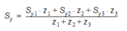
Equation 34.01

where z is the thickness of the geologic layer within the numerical cell.

Conductivity values

Hydraulic conductivity is a special parameter because it can vary by many orders of magnitude over a space of a only few metres or even centimetres. This necessitates some special interpolation strategies.

• Horizontal Interpolation

The horizontal interpolation of hydraulic conductivity interpolates the raw data values. Thus, in Step 1 above, when interpolating point values that range over several orders of magnitude, such as hydraulic conductivity, the interpolation methods will strongly weight the larger values. That is, small values will be completely overshadowed by the large values.

In fact, the interpolation in this case should be done on the logarithm of the value and then the cell values recalculated. Until this option is available in the user interface, you should interpolate conductivities outside of MIKE SHE using, for example, Surfer. Alternatively, the point values could be input as logarithmic values and the Grid Calculator Tool in the MIKE SHE Toolbox can be used to convert the logarithmic values in the .dfs2 file to conductivity values.

• Vertical Interpolation

In Step 2 above, the geologic model is scanned down and interpreted to the model cell. Although, horizontal conductivity can vary by several orders of magnitude in the different geologic layers that are found in a model cell, the water will flow horizontally based on the highest transmissivity. Thus, the averaging of horizontal conductivity can be down the same as in the example for Specific Yield above. Vertical flow, however, depends mostly on the lowest hydraulic conductivity in the geologic layers present in the model cell. In this case a harmonic weighted mean is used instead. For a 3 layer geologic model in one model cell, the vertical conductivity would be calculated by

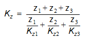
Equation 34.02

where z is the thickness of the geologic layer within the numerical cell.

2. Lenses

In building a geologic model, it is typical to find discontinuous layers and lenses within the geologic units. The MIKE SHE setup editor allows you to specify such units - again independent of the numerical model grid.

Lenses are also a very useful way to define a complex geology. In this case, the lenses are used to define the subsurface geologic units within a larger regional geologic unit.

Lenses are specified by defining either a .dfs grid file or a polygon .shp file for the extents of the lenses. The .shp file can contain any number of polygons, but the user interface does not use the polygon names to distinguish the polygons. If you need to specify several lenses, you can use a single file with many polygons and specify distributed property values, or you can specify multiple individual polygon files, each with unique property values.

In the case of lenses, an extra step is added to the beginning of the 2-step process outlined in the previous section. The location of the lenses is first interpolated to the horizontal numerical grid. Then the lenses become essentially extra geologic layers in the columns that contain lenses. However, there are a number of special considerations when working with lenses in the geologic model.

• Lenses override layers

That is, if a lense has been specified then the lense properties take precedence over the layer properties and a new geologic layer is added in the vertical column.

• Vertically overlapping lenses share the overlap

If the bottom of lense is below the top of the lense beneath, then the lenses are assumed to meet in the middle of the overlapping area.

• Small lenses override larger lenses

If a small lense is completely contained within a larger lense the smaller lense dominates in the location where the small lense is present.

• Negative or zero thicknesses are ignored

If the bottom of the lense intersects the top of the lense, the thickness is zero or negative and the lense is assumed not to exist in this area.