Prepare Land Use Inputs

The next step is the preparation of land use related model inputs. Return to the QGIS project, where the required MIKE SHE input layers will be derived from an existing land cover database.

The primary outputs required for MIKE SHE are:

• A Vegetation Map describing the spatial distribution of vegetation types used by the evapotranspiration module.
• A Manning Map describing the spatial distribution of overland flow roughness coefficients.

The first task is to identify an appropriate land cover dataset for the study area.

In this example, the Copernicus CORINE Land Cover (CLC) 2018 database is used, which provides harmonized land cover information across Europe (available from the Copernicus Land Monitoring Service).

Before preparing the MIKE SHE inputs, the original land cover classes should be reviewed using the official CLC nomenclature.

In many cases, it is beneficial to simplify the classification scheme by merging similar land cover classes.

Categories with comparable:

• vegetation properties,
• rooting characteristics,
• seasonal behaviour,
• surface roughness characteristics,

can often be represented by the same vegetation type and Manning coefficient.

This simplification reduces model complexity and parameter uncertainty while maintaining the dominant hydrological behaviour of the catchment.

The final classification should therefore reflect the hydrological processes relevant to the modelling objectives rather than the full thematic detail of the original land cover dataset.

---

Prepare the Land Use Layer

The original CORINE Land Cover dataset covers a much larger area than required for the model setup. Therefore, the first step is to reproject the dataset to the project coordinate reference system and subsequently clip it to the previously created Data_Collection_Mask.

1. Load the following layers into QGIS:

2. The CLC_2018 polygon layer.

3. The Data_Collection_Mask polygon.

4. Open the Processing Toolbox by selecting Processing → Toolbox.

5. Search for and open the Reproject Layer tool.

6. Set:

7. Input layer = CLC2018

8. Target CRS = Project coordinate reference system

   

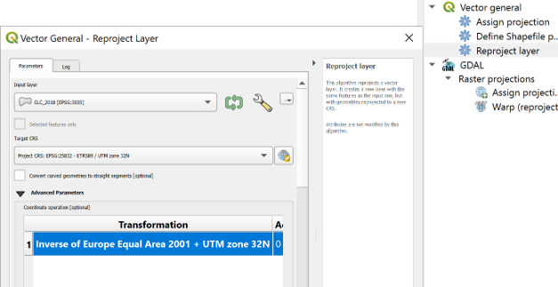
9. Specify an output file location and click Run.

10. Verify that the resulting layer uses the same coordinate reference system as the remaining model inputs.

11. Search for and open the Clip tool.

12. Set:

13. Input layer = Projected

14. Overlay layer = Data_Collection_Mask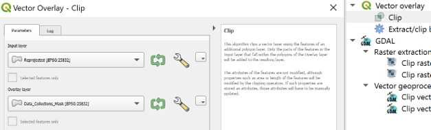

15. Specify an output file location and click Run.

16. Save the resulting layer as:

Input/LandUse/CLC_2018_clip.shp

1. Verify that the resulting polygon layer covers the complete model domain extent.

2. Continue with the parameter assignment and vegetation classification steps using the clipped layer.

---

Attach Hydrological Parameters to the Land Use Layer

The original CLC classes contain only land cover information and must therefore be supplemented with hydrological model parameters.

In this example, an external lookup table stored in Excel is used to assign:

• Simplified vegetation classes for the MIKE SHE vegetation map.
• Manning numbers for overland flow calculations.
• Subsurface leakage coefficients for limiting infiltration in sealed or highly impervious urban areas.

The lookup table contains the following fields:

Field	Description
CLC18	Original CORINE land cover code
Gridcode	Simplified vegetation class identifier
DHI_Vegetation_Type	Vegetation type used by the MIKE SHE evapotranspiration module
Manning	Manning roughness number used by the Overland Flow module
SubSurf	Subsurface leakage coefficient used to limit infiltration through paved or sealed surfaces

Typical examples include:

CLC18	CORINE Class	Simplified Class	Gridcode	Vegetation Type	Manning	Subsurface Leakage
111	Continuous urban fabric	Building	14	Water_NoVeg	28	1.00E-06
112	Discontinuous urban fabric	Residential Area	13	Residential_Area	28	1.00E-05
122	Road and rail networks	Streets	15	Water_NoVeg	50	1.00E-07
211	Non-irrigated arable land	Agriculture	11	Agriculture_Grain	5
231	Pasture and meadows	Greenlands	10	Greenlands	15
311	Broad-leaved forest	Forest deciduous	7	Forest_deciduous	12
312	Coniferous forest	Forest coniferous	5	Forest_coniferous	12
331	Beaches, dunes and sand plains	No vegetation	1	Water_NoVeg	6

---

Join the Lookup Table

1. Add the Excel lookup table to the QGIS project:

Layer → Add Layer → Add Vector Layer

1. Open the properties of the clipped CLC layer:

Right-click layer → Properties

1. Navigate to:

Joins → Add Join 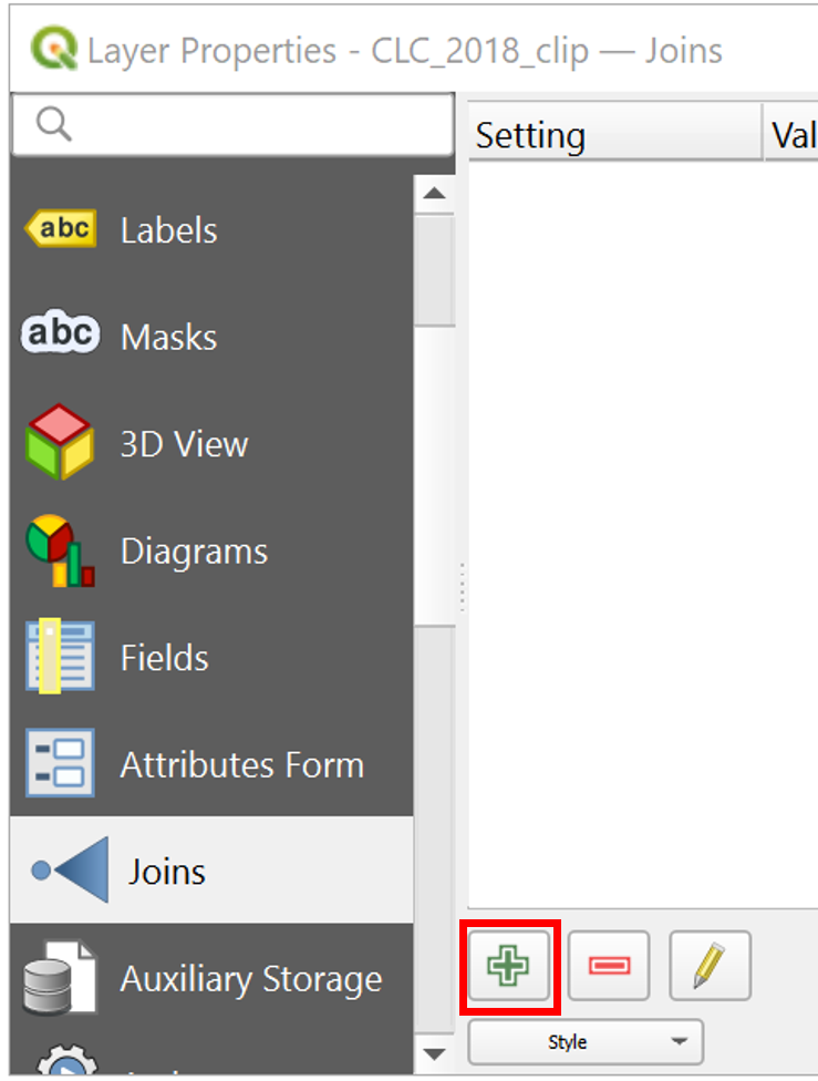4. Configure the join:

• Join layer = Land use lookup table
• Join field = CLC18

• Target field = CLC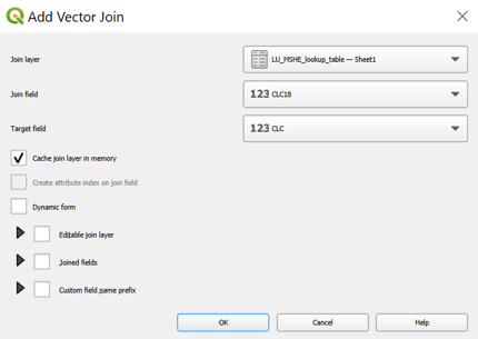

  5. Click OK.

• Open the attribute table of the clipped CLC layer and verify that the following fields have been added successfully:

• Gridcode

• DHI_ENG_ETV
• Manning

• SubSurf

• Save the joined layer as a permanent dataset. 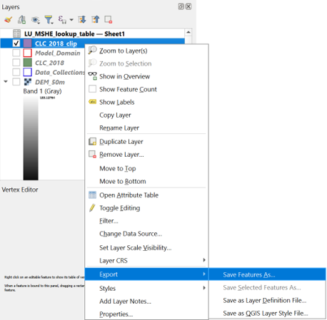This layer will subsequently be used to generate:

• the MIKE SHE vegetation map,

• the Manning roughness map,
• the subsurface leakage coefficient map.

Rasterize the Land Use Parameters

The prepared land use polygon layer can now be converted into raster inputs for MIKE SHE.

Separate raster files will be created for:

• Vegetation classes using the Gridcode field.
• Manning numbers using the Manning field.
• Subsurface leakage coefficients using the SubSurf field.

All rasters will be created using the extent of the Data_Collection_Mask and a cell size of 50 m.

---

Check the Attribute Values

1. Open the attribute table of the prepared land use layer.

2. Verify that the required fields contain valid values:

3. Gridcode

4. Manning

5. SubSurf

6. Check for empty or NULL values.

Right click on the layer → Open Attribute Table

1. Replace missing values where necessary before rasterization.

Each model cell should receive an appropriate value unless a NoData cell is intentionally required (e.g. for the subsurface leakage coefficient).

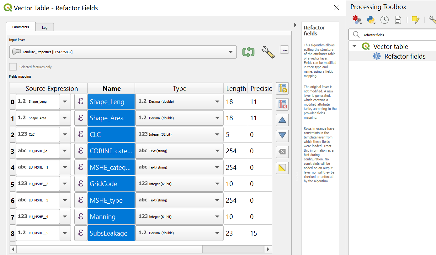
1. If necessary, field names can be renamed using the Refactor Fields tool.

---

Create the Vegetation Raster

1. Open the Processing Toolbox.

Processing → Toolbox

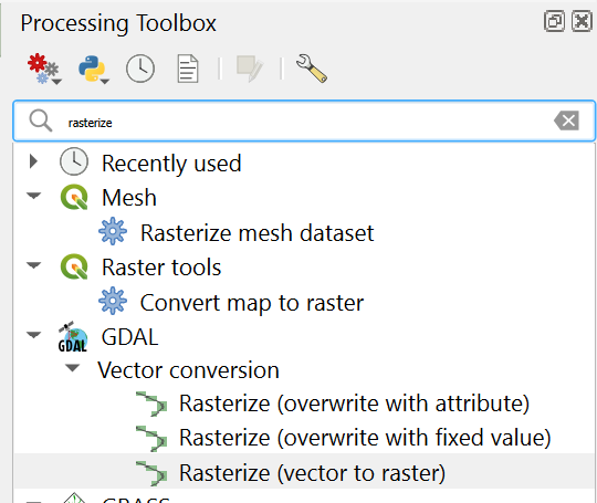
1. Search for and open:

Rasterize (vector to raster)

1. Set the following parameters:

2. Input layer = prepared land use polygon layer

3. Field to use for a burn-in value = Gridcode
4. Output raster size units = Georeferenced units
5. Horizontal resolution = 50
6. Vertical resolution = 50
7. Output extent = extent of the Data_Collection_Mask

8. Assign a specified NoData value to output bands = select an appropriate NoData value if required

9. Specify the output location and save the result, for example as:

Landuse_Gridcode.tif

1. Click Run.

Create the Manning Raster

1. Run Rasterize (vector to raster) again as described in the Land Use section.

2. Use the same settings, but select:

3. Field to use for a burn-in value = Manning

4. Save the output as:

Manning.tif

---

Create the Subsurface Leakage Raster

1. Run Rasterize (vector to raster) again as described in the Land Use section.

2. Use the same settings, but select:

3. Field to use for a burn-in value = SubSurf

4. Save the output as:

Subsurface_Leakage.tif

---

Export the Rasters to ASCII Grid Format

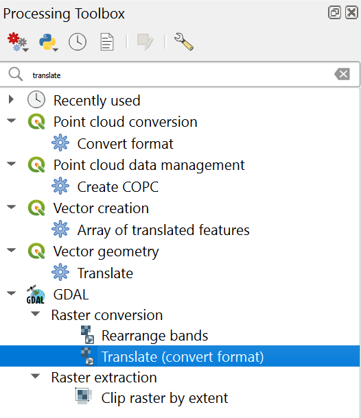
1. Open the Translate (Convert Format) tool from the Processing Toolbox.

1. Select the generated raster as the input layer.

2. Specify the output format as Arc/Info ASCII Grid.

3. Save the output with the .asc extension, for example:

4. Landuse_Gridcode.asc

5. Manning.asc

6. Subsurface_Leakage.asc

7. Repeat the conversion for all three raster layers.

8. Verify each ASCII raster:

9. The coordinate reference system matches the project CRS.

10. The cell size is 50 m.
11. The extent matches the Data_Collection_Mask.
12. The number of rows and columns is consistent between all raster layers.
13. The raster values correspond to the selected source field.
14. No unintended NoData areas occur within the model input area.

Note

The vegetation raster should normally contain integer category codes.

Manning numbers and subsurface leakage coefficients may require floating-point output values.

Verify the output data type in the rasterization settings, particularly for small leakage coefficients such as 1.0E-07.

---

Convert the Vegetation Map to DFS2 Format

The vegetation raster can now be converted to DFS2 format using the same procedure previously described for the topography raster.

1. Open MIKE Zero Toolbox.

2. Navigate to:

GIS
└── Grid2Mike

1. Select the input file:

Landuse_Gridcode.asc

Ensure that the file is not open in any other application.

If the raster is currently loaded in QGIS, remove it from the project before running Grid2Mike.

1. Select the map projection corresponding to the coordinate reference system used in the MIKE SHE model.

Recommended: Local Coordinates.

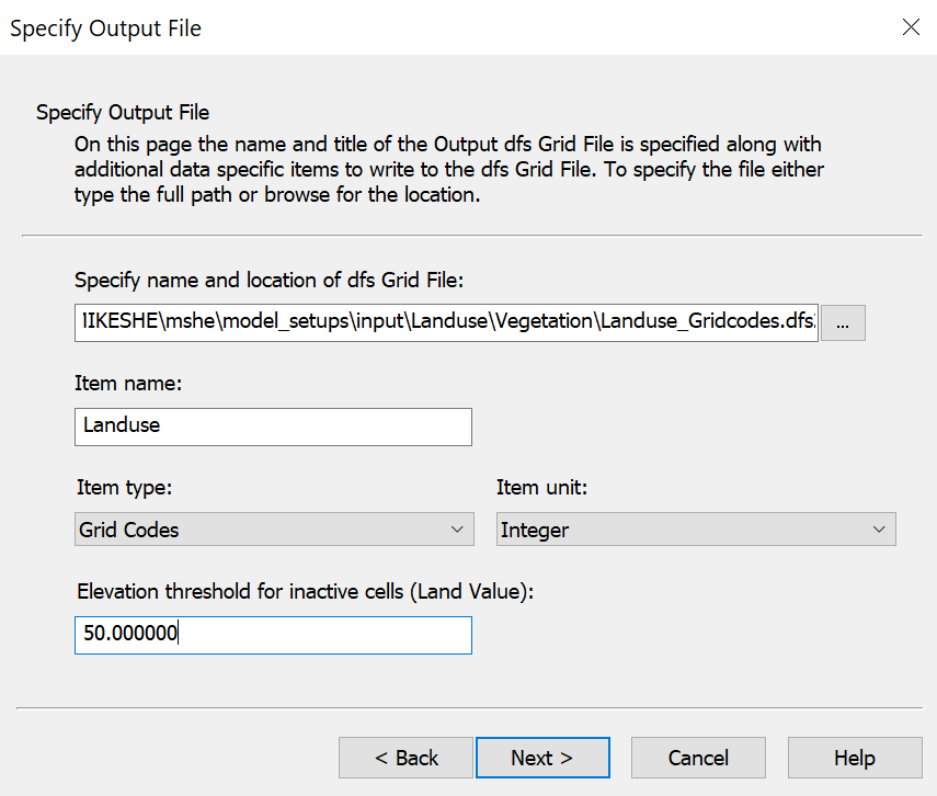
1. Specify the output file:

Input/
└── LandUse
    └── Vegetation
        └── Landuse_Gridcodes.dfs2

1. Define the item properties:

Parameter	Value
Item Name	Landuse
Item Type	Grid code
Item Unit	Integer

1. Review the settings and click Execute.

2. Open the generated DFS2 file in the Grid Editor and verify:

3. The extent matches the Data_Collection_Mask.

4. The cell size is 50 m × 50 m.
5. The raster values match the original ASCII file.

Note

The vegetation DFS2 contains integer category identifiers rather than physical quantities.

The actual vegetation properties, such as LAI, root depth, root distribution, crop coefficients, and interception storage, will be defined later in the MIKE SHE Vegetation Database using these identifiers.

Convert the Manning Map to DFS2 Format

1. Open:

GIS
└── Grid2Mike

1. Select the input file:

Manning.asc

Ensure that the file is not open in any other application.

If the raster is currently loaded in QGIS, remove it from the project before running Grid2Mike.

1. Use the same projection settings as previously described.

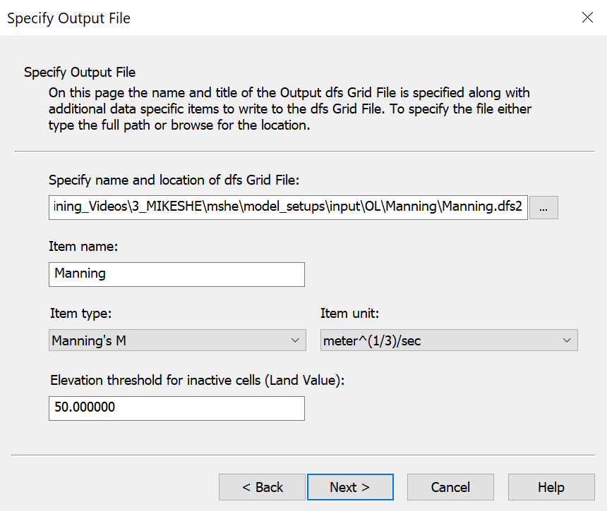
2. Specify the output file:

Input/
└── OL
    └── Manning
        └── Manning.dfs2

1. Define the item properties:

Parameter	Value
Item Name	Manning
Item Type	Manning's M
Item Unit	meter^(1/3)/s

1. Execute the conversion.

2. Open the generated DFS2 file in the Grid Editor and verify:

3. The extent matches the Data_Collection_Mask.

4. The cell size is 50 m × 50 m.
5. The raster values match the original ASCII file.

---

Convert the Subsurface Leakage Map to DFS2 Format

1. Open:

GIS
└── Grid2Mike

1. Select the input file:

Subsurface_Leakage.asc

Ensure that the file is not open in any other application.

If the raster is currently loaded in QGIS, remove it from the project before running Grid2Mike.

1. Use the same projection settings as previously described.

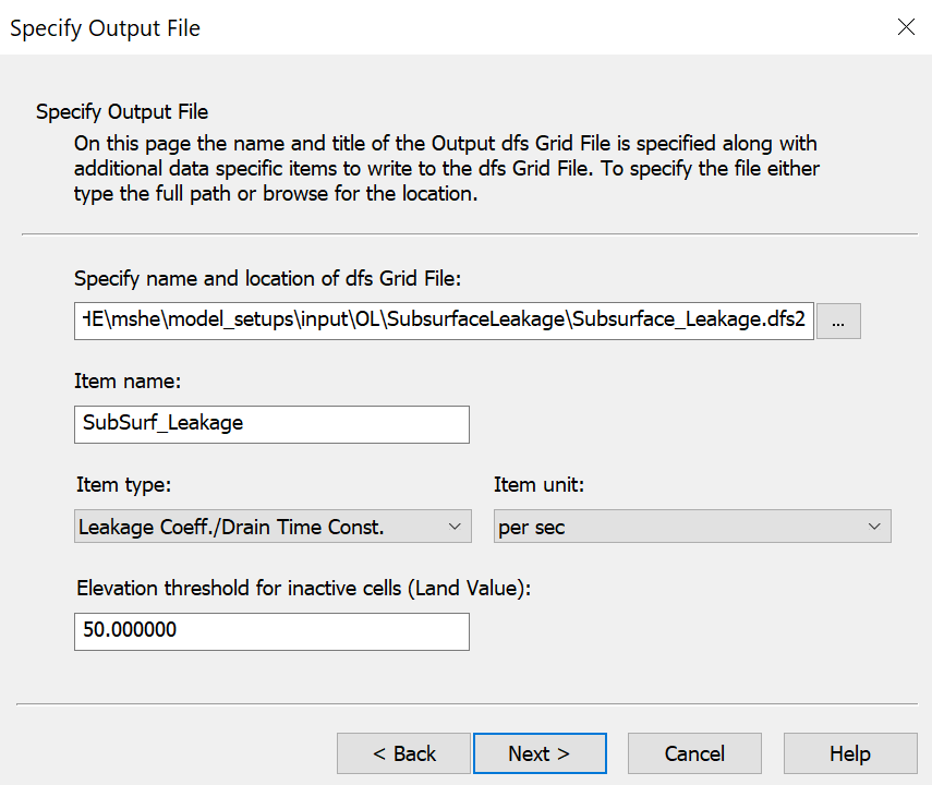
2. Specify the output file:

Input/
└── OL
    └── SubsurfaceLeakage
        └── Subsurface_Leakage.dfs2

1. Define the item properties:

Parameter	Value
Item Name	SubSurf_Leakage
Item Type	Leakage Coefficient / Drain Time Constant
Item Unit	per sec

1. Review the settings and click Execute.

2. Open the generated DFS2 file in the Grid Editor and verify:

3. The extent matches the Data_Collection_Mask.

4. The cell size is 50 m × 50 m.
5. The raster values match the original ASCII file.
6. The values correspond to the original Subsurface_Leakage.asc raster.
7. Small floating-point values (for example 1.0E-07) have been preserved correctly.

Important

The leakage coefficient is stored as a floating-point value.

Always verify that the selected output data type supports the required numerical precision before running the conversion.

---

Summary

After completing the workflow, the following MIKE SHE input files should be available:

Input/
├── LandUse
│   └── Vegetation
│       └── Landuse_Gridcodes.dfs2
└── OL
    ├── Manning
    │   └── Manning.dfs2
    └── SubsurfaceLeakage
        └── Subsurface_Leakage.dfs2

These three DFS2 files provide the spatially distributed input for:

• Vegetation classes
• Manning roughness coefficients
• Subsurface leakage coefficients

and can now be referenced by the corresponding MIKE SHE model components.

---

Click here to jump to the next section:

Implement the soil types ⬇